How Accurate Are Etherscan and EthGasStation’s Ethereum Transaction Time Estimates? | HackerNoon

Table of Links

Abstract and 1 Introduction

2 Background and 2.1 Blockchain

2.2 Transactions

3 Motivating Example

4 Computing Transaction Processing Times

5 Data Collection and 5.1 Data Sources

5.2 Approach

6 Results

6.1 RQ1: How long does it take to process a transaction in Ethereum?

6.2 RQ2: How accurate are the estimates for transaction processing time provided by Etherscan and EthGasStation?

7 Can a simpler model be derived? A post-hoc study

8 Implications

8.1 How about end-users?

9 Related Work

10 Threats to Validity

11 Conclusion, Disclaimer, and References

A. COMPUTING TRANSACTION PROCESSING TIMES

A.1 Pending timestamp

A.2 Processed timestamp

B. RQ1: GAS PRICE DISTRIBUTION FOR EACH GAS PRICE CATEGORY

B.1 Sensitivity Analysis on Block Lookback

C. RQ2: SUMMARY OF ACCURACY STATISTICS FOR THE PREDICTION MODELS

D. POST-HOC STUDY: SUMMARY OF ACCURACY STATISTICS FOR THE PREDICTION MODELS

6.2 RQ2: How accurate are the estimates for transaction processing time provided by Etherscan and EthGasStation?

Motivation. Given the lack of guarantees regarding transaction processing times in Ethereum, estimators have become a central tool for users of the platform (e.g., ÐApp developers). EthGasStation is the most popular transaction processing time estimator. Popular wallets such as Metamask rely on EthGasStation to recommend gas prices for desired processing speeds. Etherscan, one of the most popular Ethereum dashboard, has also recently developed its own processing time estimator. Despite the popularity and relevance of these estimators, their accuracy has never been empirically investigated.

Approach. As outlined in Section 5, we obtain four processing time predictions, two from EthGasStation (Gas Price API and Prediction Table API) and two from Etherscan (Pending Transaction page and the Gas Tracker). Since we know the actual processing time of each studied transaction, we can determine the accuracy of each of the four models. More specifically, for each studied transaction, we calculate the absolute error (𝐴𝐸 = |𝑎𝑐𝑡𝑢𝑎𝑙 − 𝑝𝑟𝑒𝑑𝑖𝑐𝑡𝑒𝑑|) produced by each model. We then rank the four models based on their AE distributions.

To rank the AE distributions, we follow a three-step approach. In the first step, we statistically analyze the distributions using the same standard approach as that used in RQ1: an omnibus test (Kruskal-Wallis) followed by a post-hoc test (Dunn’s test with Bonferroni correction) alongside an effect size calculation (Cliff’s Delta). We use 𝛼 = 0.05 for all tests. In the second step, we define pairwise win and draw relationships based on the results from Dunn’s test and Cliff’s Delta. We say that one model wins against another when its AE distribution is smaller than that of the other model (Dunn’s p-value < 𝛼 with a negative non-negligible effect size). Otherwise, we say that there is a draw between the two models (e.g., no statistically significant difference between the two AE distributions). In the third step, we rank the models based on the obtained win and draw relationships. Our ranking adheres to two guiding principles: (i) more wins should make a model rank higher and (ii) winning against a model that has many victories should also make a model rank higher. Fortunately, a direct parallel can be drawn between our guiding principles and the Alpha centrality. Graph centrality measures define the importance of a node in a graph [33]. The Alpha centrality assigns high scores to nodes that have many incoming connections, as well as to those that have an incoming connection from a node that has a high score itself (a recursive algorithm in nature) [7]. In other words, the Alpha centrality assigns scores to nodes in a graph based on the idea that incoming connections from high-scoring nodes contribute more to the score of the node in question than equal incoming connections from low-scoring nodes. Alpha centrality is an adaptation of the more popular Eigenvector centrality (the latter has several limitations when applied to directed graphs) [7].

In light of the aforementioned observations regarding Alpha centrality, we rank our models in the third step of our approach as follows: (a) we build a directed graph where nodes represent models, (b) we add an edge with weight 1.0 from model 𝑚2 to model 𝑚1 when 𝑚1 wins against 𝑚2 (see the definition of win), (c) we add an edge with weight 0.5 from 𝑚1 to 𝑚2 and vice-versa when there is a draw between 𝑚1 and 𝑚2 (see the definition of draw), (d) we calculate the Alpha centrality of each model in the graph[15], and (e) we assign ranks to models in accordance to their centrality score (the model with highest centrality score is assigned rank 1, the model with second highest centrality score is assigned rank 2, and so forth). The rationale behind the weights in (b) and (c) is to enforce that wins count more than draws.

Finally, for information purposes, we also summarize the accuracy of the four model in terms of four accuracy measures, namely: Mean Absolute Error (MAE), Median Absolute Error (MedAE), Mean Absolute Percentage Error (MAPE), and Median Absolute Percentage Error (MedAPE).

Findings. Observation 7) At the global level, the four prediction models are equivalent. The four models have roughly similar median AEs, which range from 40.8s to 58.2s (see Table 8 in Appendix C for additional performance statistics). We ran our ranking procedure and obtained an identical rank for all models. Upon closer inspection, we observed a statistically significant difference between all pairs of models. Nonetheless, the magnitude of the effect sizes was negligible in all cases. Therefore, we consider the four models to have equivalent prediction accuracy at the global level.

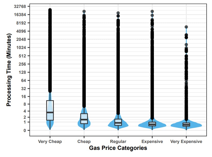
Observation 8) When stratifying the analysis by gas prices categories, the Etherscan Gas Tracker webpage outperforms the others for “very cheap” and “cheap” transactions. In turn, the EthGasStation Gas Price API outperforms the others for the remaining gas price categories. In RQ1, we observed that there is noticeably more variability in the processing time for very cheap and cheap transactions (Figure 6). This means that cheaper transactions are inherently harder to predict compared to more expensive transactions. Therefore, we decided to reassess the four prediction models on a per gas-price-category basis (i.e., a stratified analysis). The results that we obtained from running our ranking approach are shown in Table 6. We use shading to indicate the best performing model(s) for each gas price category.

Analysis of Table 6 reveals that the Etherscan Gas Tracker webpage outperforms the four other models for the very cheap and cheap gas price categories. In all remaining price categories, the EthGasStation Gas Price API is the best model (with ties for the very expensive category). In other words, if ÐApp developers wish to maximize prediction accuracy using the state-of-the-practice models, they would need to use two models that belong to different online estimation services.

If developers only care about the prediction of cheaper priced transactions (the hardest ones to predict), then they can rely on the Etherscan Gas Tracker webpage alone. However, we highlight once again that such a model is a black box (see Section 5). For instance, Etherscan does not provide any public documentation concerning the design of this model and how it operates. A summary of accuracy statistics for the four models on a per gas-price-category basis can be found in Appendix C.

[15] We use the alpha_centrality function from the igraph R package (version 1.2.5): https://cran.r-project.org/web/pack ages/igraph.