How Long Does It Take To Process a Transaction in Ethereum? | HackerNoon

Table of Links

Abstract and 1 Introduction

2 Background and 2.1 Blockchain

2.2 Transactions

3 Motivating Example

4 Computing Transaction Processing Times

5 Data Collection and 5.1 Data Sources

5.2 Approach

6 Results

6.1 RQ1: How long does it take to process a transaction in Ethereum?

6.2 RQ2: How accurate are the estimates for transaction processing time provided by Etherscan and EthGasStation?

7 Can a simpler model be derived? A post-hoc study

8 Implications

8.1 How about end-users?

9 Related Work

10 Threats to Validity

11 Conclusion, Disclaimer, and References

A. COMPUTING TRANSACTION PROCESSING TIMES

A.1 Pending timestamp

A.2 Processed timestamp

B. RQ1: GAS PRICE DISTRIBUTION FOR EACH GAS PRICE CATEGORY

B.1 Sensitivity Analysis on Block Lookback

C. RQ2: SUMMARY OF ACCURACY STATISTICS FOR THE PREDICTION MODELS

D. POST-HOC STUDY: SUMMARY OF ACCURACY STATISTICS FOR THE PREDICTION MODELS

6 RESULTS

6.1 RQ1: How long does it take to process a transaction in Ethereum?

Motivation. In Ethereum, users (e.g., developers) interact with the blockchain via transactions. Developers of ÐApps want the transactions issued by their applications to be processed as quickly as possible in order to deliver a pleasant end-user experience. Yet, ÐApp developers need to pay for these transactions by assigning a certain gas price to them. That is, ÐApp developers need to find the optimal balance between cost (transaction fees) and end-user experience (transaction processing times). Nonetheless, to this day, there is little empirical evidence to guide developers in making informed decisions regarding the gas price of transactions. Even simple statistics such as the typical processing time of transactions have been little investigated.

Approach. As described in Section 5 and summarized in Figure 3, we collect transaction processing times from Etherscan. In this RQ, we statistically analyze the distribution of transaction processing times and determine how gas prices influence these times. More specifically, we classify the gas prices of the studied transactions into five categories, namely: very cheap, cheap, regular, expensive, and very expensive. The ranges of gas prices for these categories are determined dynamically. More specifically, the gas price category of each studied transaction 𝑡 is determined by (i) taking the gas price of all transactions included in the 120 blocks that precede the block containing 𝑡 (see Appendix B.1 for details), (ii) splitting the price distribution into five equal parts (quintiles), (iii) assigning a gas price category to each quintile (first quintile and lower represents very cheap, second quintile represents cheap, and so on), and finally (iv) mapping the gas price of 𝑡 to one of the quintiles.

We perform statistical tests to compare multiple distributions. We perform a standard statistical procedure, which consists of running an omnibus test (Kruskal-Wallis), followed by a post-hoc test (Dunn’s test) with effect size calculation (Cliff’s Delta). By means of this procedure, we can determine whether there is a statistically significant difference between a given pair of distributions (e.g., the processing times associated with expensive and very expensive price categories) and, in the positive case, determine whether such a difference is meaningful in practice.

More specifically, first we run the Kruskal-Wallis test (𝛼 = 0.05). The Kruskal-Wallis test is the non-parametric equivalent of the one-way analysis of variance (ANOVA). We use the Kruskal-Wallis test to determine whether at least one of the distributions differs from the others with statistical significance. In the positive scenario, we then run the Dunn’s post-hoc test (𝛼 = 0.05) with Bonferroni correction. Dunn’s test performs multiple pairwise distribution comparisons. The null hypothesis for each pairwise comparison is that the probability of observing a randomly selected value from the first distribution that is larger than a randomly selected value from the second distribution equals one half (i.e., the same null hypothesis as that of the Wilcoxon signed-rank test). If we observe a statistically significant difference between a given pair of distributions, we calculate the Cliff’s Delta (𝛿) effect size measure in order to better understand the practical significance of the difference. Given two distributions 𝑑1 and 𝑑2, Cliff’s Delta measures how often the values from 𝑑1 are larger than those from 𝑑2. We assess Cliff’s Delta using the following thresholds [37]: negligible for |𝛿 | ≤ 0.147, small for 0.147 < |𝛿 | ≤ 0.33, medium for 0.33 < |𝛿 | ≤ 0.474, and large otherwise.

Findings. Observation 1) Transactions take a median of 57s to be processed. Figure 4 depicts the distribution of transaction processing times. Three quarters of the processing times lie in the range of 33s to 2m 23s (interquartile). As another reference point, 90% of the transactions are processed within 8m.

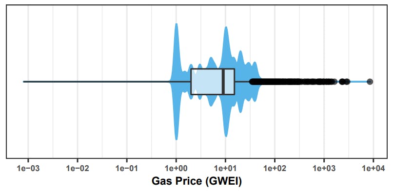
Observation 2) Median-priced transactions (9 GWEI) are processed within 3m 04s in 90% of the cases. The distribution of gas prices is shown in Figure 5. Three quarters of the gas prices lie in the range of 2.0 to 15.2 GWEI range (interquartile).

The violin plot suggests that there are specific values for gas price that are recurrently used (e.g., notice the blobs around 1 GWEI and 10 GWEI). Hence, in Table 3 we show the top-5 most common gas prices and their associated 90th percentile processing time. For instance, 90% of the transactions priced at 1 GWEI are processed within 56m 41s (≈ 1 hour).

Observation 3) Very cheap, cheap, regular, expensive, and very expensive are processed within 50m 43s, 05m 36s, 03m 02s, 01m 32s, and 01m 08s respectively in 90% of the cases. Table 4 shows gas price statistics for each of the five gas price categories that we defined. Such statistics provide an intuition as to what is considered cheap and expensive in Ethereum during the studied period. Furthermore, Table 4 indicates the 90th percentile processing time for each gas price category. ÐApp developers can leverage the information shown in Table 4 to make more informed gas price choices. Figure 21 in Appendix B depicts the distribution of gas prices for each of our gas price categories.

Observation 4) Higher gas prices result in faster transaction processing times with diminishing returns. Figure 6 depicts the processing times for each gas price category. The plots indicate that processing times decrease as prices increase (e.g., compare very expensive to very cheap). Nevertheless, the return over investment diminishes as prices increase (e.g., compare expensive to very expensive).

In order to further evaluate the relation between gas prices and processing times, we computed a Kruskal-Wallis test (𝛼 = 0.05) on the distributions shown in Figure 6. The result of the test indicates that at least one of the distributions differs from the others (as we expected from a visual inspection of Figure 6). Next, we perform Dunn’s post-hoc test alongside effect size calculations in order to quantify the difference between the distributions. The results for adjacent price categories are summarized in Table 5.

The results depicted in Table 5 corroborate our claim of diminishing returns. In particular, despite the statistically significant difference flagged by the Dunn’s test, the Cliff’s Delta score indicates that the difference in processing times between expensive and very expensive is actually negligible.

Observation 5) 25% of the very cheap transactions were processed within only 1m 20s. Since miners’ revenue depend on transaction fees, transactions with lower gas prices will receive lower

priority and frequently take longer to be processed. Indeed, as depicted in Figure 6, very cheap transactions have the highest processing time median. Nevertheless, depending on contextual factors (e.g., the average gas price set by transaction issuers at a given hour of the day), very cheap transactions can be processed as fast as expensive and very expensive transactions. In particular, we observe that 25% of all very cheap transactions were processed within 1m 20s, which happens to be lower than the 90th Percentile processing time for expensive transactions. Hence, discovering the moments at which very cheap can be processed fast would bring a major financial benefit to ÐApp developers. Nevertheless, the inherent variability in the processing time of very cheap transactions makes this task far from trivial. In RQ2, we devote particular attention to how accurately online estimation services perform for very cheap transactions.

Observation 6) Even very expensive transactions can sometimes take days to be processed. Although the 90th percentile of the processing time for very expensive transactions is only 01m 08s, we note from Figure 6 that some transactions in this price category did take days to be processed. A common reason why very expensive transactions get delayed is the existence of a preceding pending transaction sent by the same transaction issuer, possibly with a cheaper price (please refer to the definition of nonce in Section 2.2). We thus conjecture that the majority of very expensive transactions that took days to be processed (i.e., outliers) were waiting for a preceding pending transaction to be processed.