


Table of Links
-
Introduction
-
Hypothesis testing
2.1 Introduction
2.2 Bayesian statistics
2.3 Test martingales
2.4 p-values
2.5 Optional Stopping and Peeking
2.6 Combining p-values and Optional Continuation
2.7 A/B testing
-
Safe Tests
3.1 Introduction
3.2 Classical t-test
3.3 Safe t-test
3.4 χ2 -test
3.5 Safe Proportion Test
-
Safe Testing Simulations
4.1 Introduction and 4.2 Python Implementation
4.3 Comparing the t-test with the Safe t-test
4.4 Comparing the χ2 -test with the safe proportion test
-
Mixture sequential probability ratio test
5.1 Sequential Testing
5.2 Mixture SPRT
5.3 mSPRT and the safe t-test
-
Online Controlled Experiments
6.1 Safe t-test on OCE datasets
-
Vinted A/B tests and 7.1 Safe t-test for Vinted A/B tests
7.2 Safe proportion test for sample ratio mismatch
-
Conclusion and References
4 Safe Testing Simulations
4.1 Introduction
In this section, we compare the classical t-test with the safe t-test, and the χ2 test with the safe proportion test. A thorough library for safe testing has been developed in R [LTT20]. With the goal of increasing adoption in the field of data science, we ported the code for the safe t-test and the safe proportion test into Python.
4.2 Python Implementation
While the logic of the safe t-test remains the same, there were a number of inefficiencies in the original code that needed to be addressed in order to work with large sample sizes. The improvements are detailed here.
The first improvement comes in determining the sample size required for a batch process of the data. The original function performs a linear search from 1 to an arbitrary high number. For each possible sample size in the range, the function calculates the E-value based on the sample sizes, degrees of freedom, and the effect size. The loop breaks when the E-value is greater than 1/α. Since this is a monotonically increasing function, a binary search speeds up the calculation considerably, reducing the computational complexity from O(n) to O(log n). This optimization proved to be necessary when working with millions of samples.
The next speed improvement necessary is calculating the stopping time for a power of 1 − β. This is determined through simulation of data differing by the minimal effect size. Over the course of N simulations, data of length m are individually streamed to determine the point at which the E-value crosses 1/α. Once again, this process is done through a linear search. To optimize this function, the calculation of the martingale is parallelized over the whole vector of length m. The computational complexity remains O(Nm), but the vector computation takes place in Numpy code, as opposed to a Python loop. Numpy code is written in C, hence the calculation is much faster.
The final modification is not in reducing computational complexity, but in improving the capabilities of the safe proportion test. This test was written in R as a two-sample test with fixed batch sizes. For our use case, a one-sample test with variable batch sizes was required to detect sample mismatch ratio, and was therefore developed for the Python package.
4.3 Comparing the t-test with the Safe t-test
The most straightforward way to understand the safe t-test is to compare it with its classical alternative. We perform simulations of an effect size δ and a null hypothesis H0 : δ = 0. Setting the significance level α = 0.05 we can simulate an effect size δ between two groups to determine when the test is stopped. If the simulated E-value crosses 1/α = 20, the test is stopped with H0 rejected. If no effect is detected, the test is stopped at a power of 1 − β = 0.8, as this power is common within industry. Figure 3 shows simulations of stopping times and decisions of the safe test compared to the t-test.


As we can see from the average stopping times in Figure 3, the safe t-test uses fewer than 500,000 samples to deliver statistically valid results, while the classical t-test requires over 600,000. However, the sample size required to reach 1 − β power for the safe t-test is approximately 850,000, much larger than that of the classical t-test. One may ask whether it is acceptable to simply conduct the safe t-test until the classical t-test sample size. Figure 4 (left) shows the impact of this action on the statistical errors. By the completion of the test, both the classical t-test and the safe t-test are meeting the requirement that the Type I errors are below α = 0.05 and the Type II errors are below β = 0.2. However, combining the two tests results in an inflated Type I error rate, and hence will not meet the experimenter’s expected level of statistical significance. Given the savings in test duration, there may be motivation to develop methods combine these tests in the future such that the false positive rate remains below α, for example using the Bonferroni correction.
As well as the overall conclusions of the two tests, it is interesting to consider the experiments for which the classical t-test and the safe t-test disagree. As seen in Figure 4 (right), while both tests achieve 80% power, they do so in very different ways. Many simulations for which the classical t-test accepts H0 are rejected by the safe t-test, and vice versa. This difference in outcomes will likely be difficult to internalize for practitioners who consider


the t-test to be the source of truth for their platform.
While Figure 3 evaluates safe stopping times for a fixed effect size, it is important to consider the results for a wide range of effect sizes. To aggregate the results of effect sizes from 0.01 to 0.3, we normalize the stopping times by the t-test stopping time. The results of this analysis can be seen in Figure 5.


The plot of Figure 5 shows both the average stop of the safe t-test and the sample size required for 80% power. On average, the safe test uses 18% less data than the t-test. In order to achieve the same power of 80%, however, the safe test uses 36% more data. Given that most A/B tests do not result in the rejection of H0 [Aze+20], this could result in longer experiments overall for practitioners.
4.4 Comparing the χ2 -test with the safe proportion test


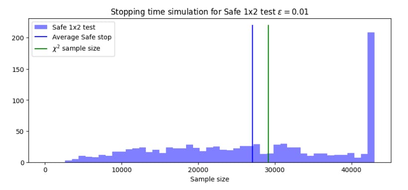
The results of Figure 6 are remarkably similar to those seen comparing the t-test and the safe t-test in Figure 3. The safe test again uses fewer samples, on average, than its classical alternative, while the maximum stopping time to achieve the required power is higher. Next, we consider the sample sizes of the tests as a function of the difference ϵ. Figure 7 shows both the average and maximum stopping times for ϵ ∈ [0001, 0.1].
As seen in Figure 7, the average sample size required for the safe proportion test is less than that of the χ2 test for all values of ϵ. This suggests that the safe proportion test will be competitive with the χ2 test, even for detecting small effects. Looking at these results, one may question whether it is appropriate to set a prior based on an unknown effect size. However, the prior can based the effect size calculated from the data after each sample. Hence, setting the priors based on the current effect size has no impact on the validity of the test.


In this section, we have compared the safe t-test and the safe proportion test with their classical alternatives. It was found that average sample sizes for the safe t-test are smaller than those of the classical t-test for a wide range of effect sizes. However, the maximum sample size can be much greater to achieve the same statistical power. Additionally, the average sample sizes of the safe proportion test are smaller than those of the χ2 test. These findings motivate further adoption of safe tests in scientific endeavours. In the next section, we compare the safe t-test to another anytime-valid test used in industry, the mixture sequential probability ratio test.
Author:
(1) Daniel Beasley
This paper is available on arxiv under ATTRIBUTION-NONCOMMERCIAL-SHAREALIKE 4.0 INTERNATIONAL license.

