


Table of Links
Abstract and 1. Introduction
-
Related Works
-
Convex Relaxation Techniques for Hyperbolic SVMs
3.1 Preliminaries
3.2 Original Formulation of the HSVM
3.3 Semidefinite Formulation
3.4 Moment-Sum-of-Squares Relaxation
-
Experiments
4.1 Synthetic Dataset
4.2 Real Dataset
-
Discussions, Acknowledgements, and References
A. Proofs
B. Solution Extraction in Relaxed Formulation
C. On Moment Sum-of-Squares Relaxation Hierarchy
D. Platt Scaling [31]
E. Detailed Experimental Results
F. Robust Hyperbolic Support Vector Machine
A Proofs
A.1 Deriving Soft-Margin HSVM with polynomial constraints
This section describe the key steps to transform from Equation (6) to Equation (7) for an efficient implementation in solver as well as theoretical feasibility to derive semidefinite and moment-sum-of-squares relaxations subsequently.
By introducing the slack variable 𝜉𝑖 as the penalty term in Equation (6), we can rewrite Equation (6) into
then by rearranging terms and taking sinh on both sides, it follows that


where the last equality follows from hyperbolic trig identities. To make it ready for moment-sum-of-squares relaxation, we turn the function into a polynomial constraint by taking the taylor expansion up to some odd orders (we need monotonic decreasing approximation to 𝑔(.), so we need odd orders).
If taking up to the first order, we relax the problem into Equation (7) [2]. If taking up to the third order, we relax the original problem to,
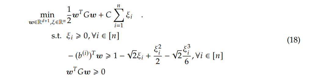

It’s worth mentioning that we expect the lower bound gets tighter as we increase the order of Taylor expansion. However, once we apply the third order Taylor expansion, the constraint is no longer quadratic, eliminating the possibility of deriving a semidefinite relaxation. Instead, we must rely on moment-sum-of-squares relaxation, potentially requiring a higher order of relaxation, which may be highly time-costly.
A.2 Stereographic projection maps a straight line on H2 to an arc on Poincaré ball B2
Suppose w = [𝑤0, 𝑤1, 𝑤2] is a valid hyperbolic decision boundary (i.e. w ∗ w < 0), and suppose a point on the Lorentz straight line, 𝑥 = [𝑥0, 𝑥1, 𝑥2] with w ∗ 𝑥 = 0, is mapped to a point, 𝑣 = [𝑣1, 𝑣2].l in Poincaré space, then we have
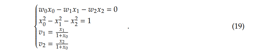

If 𝑤 > 0, we further have
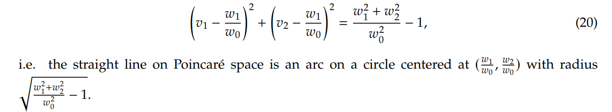

One could show that if 𝑤0 = 0, then it is the “arc” of a infinitely large circle, or just a Euclidean straight line passing through the origin with normal vector (𝑤1, 𝑤2). With this simplification, one could plot the decision boundary on the Poincaré ball easily.
:::info
Authors:
(1) Sheng Yang, John A. Paulson School of Engineering and Applied Sciences, Harvard University, Cambridge, MA (shengyang@g.harvard.edu);
(2) Peihan Liu, John A. Paulson School of Engineering and Applied Sciences, Harvard University, Cambridge, MA (peihanliu@fas.harvard.edu);
(3) Cengiz Pehlevan, John A. Paulson School of Engineering and Applied Sciences, Harvard University, Cambridge, MA, Center for Brain Science, Harvard University, Cambridge, MA, and Kempner Institute for the Study of Natural and Artificial Intelligence, Harvard University, Cambridge, MA (cpehlevan@seas.harvard.edu).
:::
:::info
This paper is available on arxiv under CC by-SA 4.0 Deed (Attribution-Sharealike 4.0 International) license.
:::
[2] note that in [4], the authors use 1 − 𝜉𝑖 instead of 1 − √ 2𝜉𝑖 . We consider our formulation less sensitive to outliers than the former formulation.


