


Table of Links
Abstract
-
Keywords and 2. Introduction
-
Set up
-
From Classical Results into Differential Machine Learning
4.1 Risk Neutral Valuation Approach
4.2 Differential Machine learning: building the loss function
-
Example: Digital Options
-
Choice of Basis
6.1 Limitations of the Fixed-basis
6.2 Parametric Basis: Neural Networks
-
Simulation-European Call Option
7.1 Black-Scholes
7.2 Hedging Experiment
7.3 Least Squares Monte Carlo Algorithm
7.4 Differential Machine Learning Algorithm
-
Numerical Results
-
Conclusion
-
Conflict of Interests Statement and References
Notes
6 Choice of Basis
A parametric basis can be thought of as a set of functions made up of linear combinations of relatively few basis functions with a simple structure and depending non-linearly on a set of “inner” parameters e.g., feed-forward neural networks with one hidden layer and linear output activation units. In contrast, classical approximation schemes do not use inner parameters but employ fixed basis functions, and the corresponding approximators exhibit only a linear dependence on the external parameters.
However, experience has shown that optimization of functionals over a variable basis such as feed-forward neural networks often provides surprisingly good suboptimal solutions.
A well-known functional-analytical fact is the employing the Stone-Weierstrass theorem, it is possible to construct several examples of fixed basis, such as the monomial basis, a set that is dense in the space of continuous function whose completion is L2. The limitations of the fixed basis are well studied and can be summarized as the following.
6.1 Limitations of the Fixed-basis
The variance-bias trade-off can be translated into two major problems:
-
Underfitting happens due to the fact that high bias can cause an algorithm to miss the relevant relations between features and target outputs. This happens with a small number of parameters. In the previous terminology, that corresponds to a low d value (see Equation 4).
-
The variance is an error of sensitivity to small fluctuations in the training set. It is a measure of spread or variations in our predictions. High variance can cause an algorithm to model the random noise in the training data, rather than the intended outputs, which is denominated as overfitting. This, in turn, happens with a high number of parameters. In the previous terminology, that corresponds to a high d value (see Equation 4).
The following result resumes the problem discussed. I will state it as in Barron, 1993, and the proof can be found in Barron, 1993 and Gnecco et al., 2012
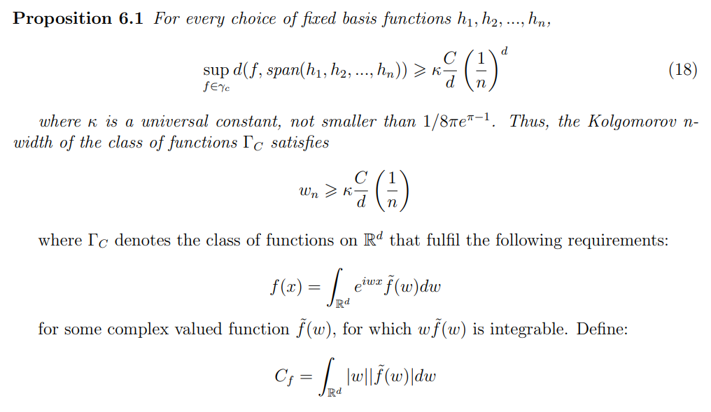

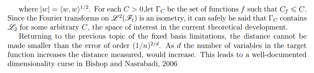

So, there is a need to study the class of basis, that can adjust to the data. That is the case with the parametric basis.
6.2 Parametric Basis: Neural Networks
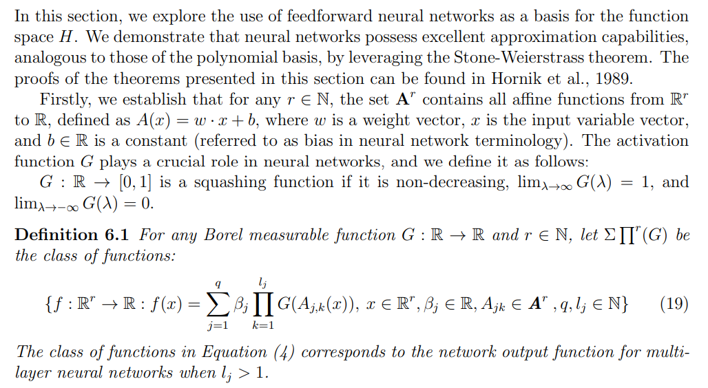

From Hornik et al., 1989, we find the following relevant results:
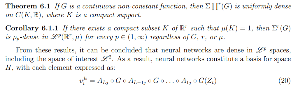

The flexibility and approximation power of neural networks makes them an excellent choice as the parametric basis.
6.2.1 Depth
In practical applications, it has been noted that a multi-layer neural network, outperforms a single-layer neural network. This is still a question under investigation, once the top-of-the-art mathematical theories cannot account for the multi-layer comparative success. However, it is possible to create some counter-examples, where the single-layer neural network would not approach the target function as in the following proposition:
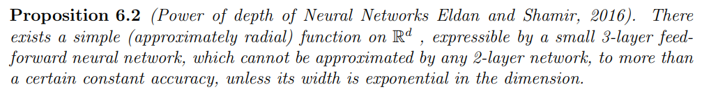

Therefore it is beneficial or at least risk-averse to select a multi-layer feed-forward neural network, instead of a single-layer feed-forward neural network
6.2.2 Width
This section draws inspiration from the works Barron, 1993 andTelgarsky, 2020. Its primary objective is to investigate the approximating capabilities of a neural network based on the number of nodes or neurons. I provide some elaboration on this result, once it is not so well known and it does not require any assumption regarding the activation function unlike in Barron, 1994.
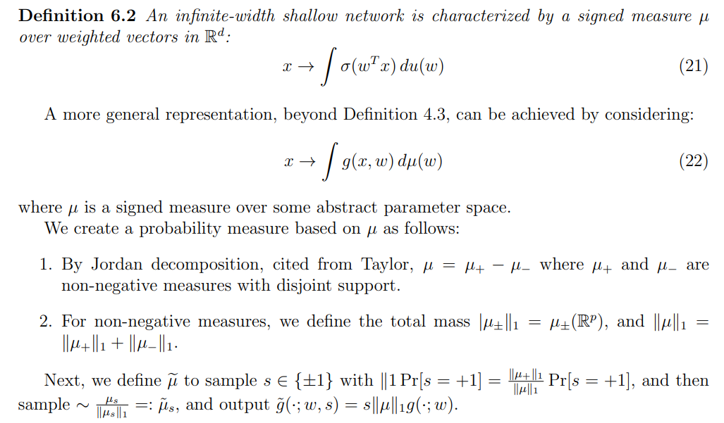

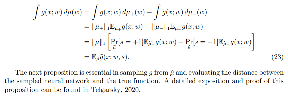
This sampling procedure correctly represents the mean as:

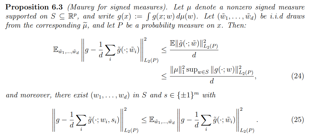

As the number of nodes, d, increases, the approximation capability improves. This result, contrary to Proposition 5.1, establishes an upper bound that is independent of the dimension of the target function. By comparing both theorems, it can be argued that there is a clear advantage for feed-forward neural networks when d > 2 for d ∈ N.
:::info
Author:
(1) Pedro Duarte Gomes, Department of Mathematics, University of Copenhagen.
:::
:::info
This paper is available on arxiv under CC by 4.0 Deed (Attribution 4.0 International) license.
:::


