


Table of Links
Abstract and 1. Introduction
- The Model Set-up
- Price Impact in a Market with No Transaction Costs
- Price Impact in a Market with Transaction Costs
Appendix A. Proofs of Section 3
Appendix B. Proofs of Section 4
References
3. Price Impact in a Market with no Transaction Costs
We are now ready to introduce the way we model investors’ price impact. For this, we first take the position of investor n and assume (for now) that she acts strategically, while the rest of the investors are price takers. This creates a best-response function that eventually leads to the Nash equilibrium when all investors apply the same strategy.
Consider again the market clearing condition (7) and assume that all the investors, besides n, act optimally through (6). In the spirit of [Ant17], we observe that market’s returns can be viewed as a function of investor n’s demand. Indeed, in this context the clearing condition is written as:
To simplify the formulas that follow, we introduce the notation for each investor’s relative risk tolerance


The following proposition deals with the solution of problem (13).
Proposition 3.1. Under Assumption 2.2, the optimization problem (13) has the following unique solution:


Henceforth, we also refer to (14) as the best-response strategy of investor n in the frictionless market.
Remark 3.2. Comparing the best-response strategy of investor n with the respective competitive optimal strategy (6) at the competitive equilibrium we directly get:

Hence, investor n has motive to decrease the volume of her demand (positive or negative) when compared to her price-taking demand. Intuitively, lower demand implies a lower equilibrium price and hence higher required return for the assets that the investor is about to buy.
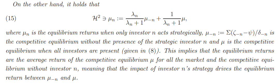

3.1. Investors’ revealed risk exposure. By applying strategy (14), investor n drives the equilibrium returns to (15), i.e. to a different equilibrium. As mentioned in the introductory section, the main reason for investors’ trading in this market is to hedge their risk exposure (the other reason is to offset noise traders’ demand). When investor n applies strategy (14), she essentially reveals different hedging needs than her true ones. In order to see that, recall the price-taking demand (6), where the risk exposure is the intercept point of the affine demand function. Under price impact, investor n submits a different demand function and hence the implied risk exposure is shifted. This creates the very useful and intuitive notion of the revealed risk exposure that is formally defined below.
Definition 3.3 (Revealed risk exposure process). For any given demand process φ ∈ H2 of investor m and local returns ν ∈ H2 pinned down at the equilibrium, the revealed exposure of investor m is defined as:
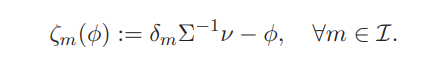

With a slight abuse of notation, we distinguish between the revealed risk exposure process ζm(·) and the true exposure process, ζm of each investor m. Departing from the above definition, we derive the following result:
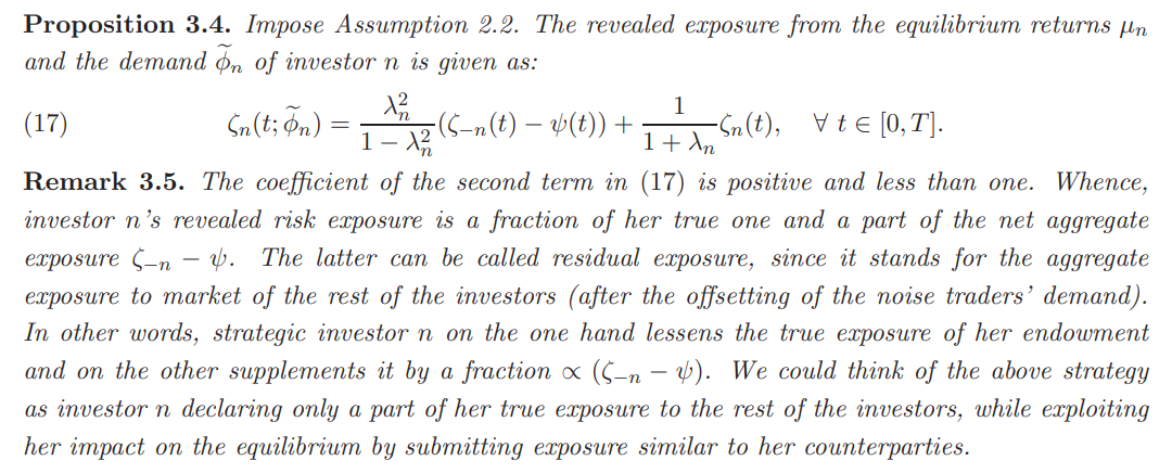

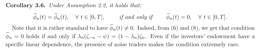
A reasonable question that arises is when does the strategic demand of an investor coincides with the competitive one. As stated in the following corollary, this coincidence never happens, as long as investor’s demand at competitive equilibrium is non-zero.

3.2. The Nash equilibrium returns in a market with no transaction costs. We now consider a market where all the investors act strategically by applying the strategy that is determined by problem (12). In the view of (16), the Nash equilibrium is induced as the fixed point of (17). We formally define the the Nash equilibrium returns in this context below:
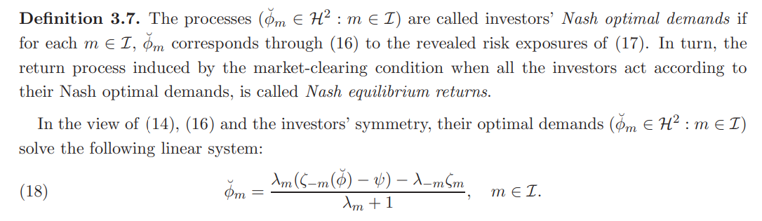

The fact that solutions to the above belong in H2 is guaranteed by Assumption 2.2 and system’s linearity. In other words, Nash equilibrium demands have the form of the best-response strategy (14), but with the rest of the investors being strategic too. Armed with the above, we give the following characterization:
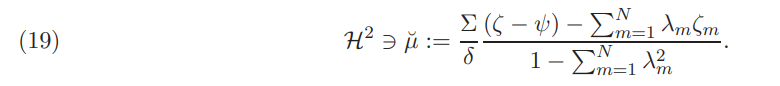
Theorem 3.8. Under Assumption 2.2, the unique Nash equilibrium returns in a market without transaction costs take the following form:

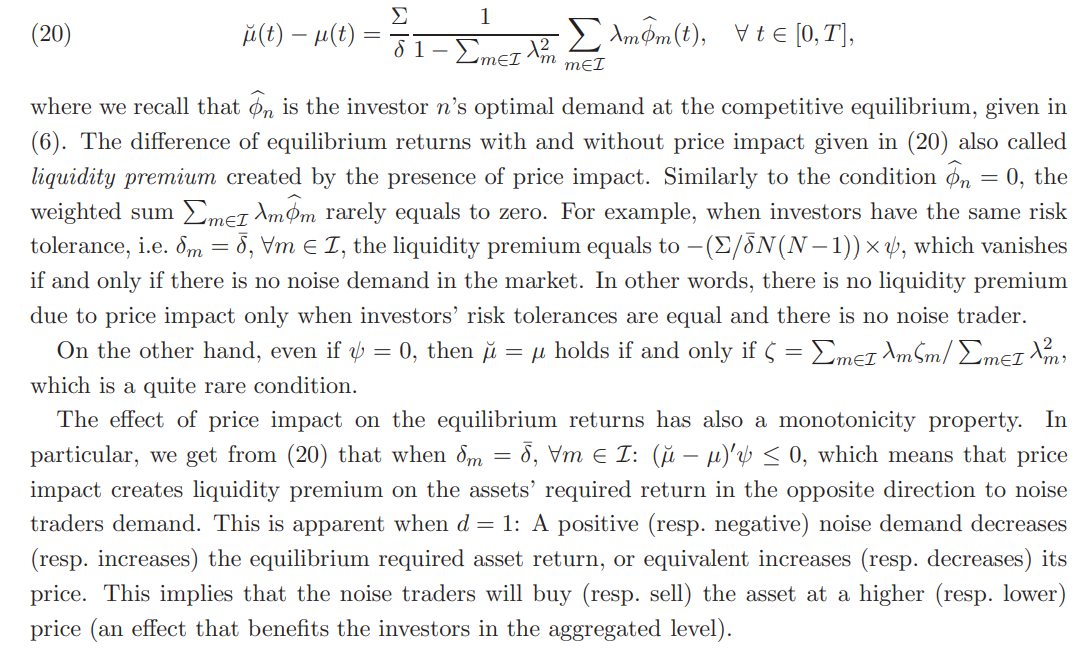
As Corollary 3.6 implies, Nash equilibrium is generally different than the competitive one. Indeed, using (8) and (19) we readily get that:

Another issue that stems from equilibria comparison is whether the utility gain (or utility surplus) that is created by the trading is higher or lower for each investor due to price impact. In general, competitive equilibrium is consistent with Pareto optimal allocation and hence another equilibrium allocation decreases the aggregate gain of utility. However, in individual level, Nash equilibrium may be beneficial for some investor(s). This feature appears in several recent non-competitive settings such as [AK24] and [MR17].
To this end, we define the utility surplus for each asset return ν ∈ H2 and each admissible strategy φ ∈ H2 of the investor m as:


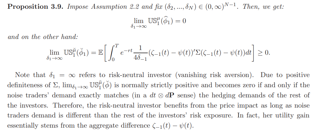
In the view of the related literature we get the following limiting result:

:::info
Authors:
(1) Michail Anthropelos;
(2) Constantinos Stefanakis.
:::
:::info
This paper is available on arxiv under CC by 4.0 Deed (Attribution 4.0 International) license.
:::


