


Table of Links
- I. Abstract and Introduction
- II. Related Work
- III. Modeling of Mobile Channels
- IV. Channel Discretization
- V. Channel Interpolation and Extrapolation
- VI. Numerical Evaluations
- VII. Conclusions, Appendix, and References
IV. CHANNEL DISCRETIZATION
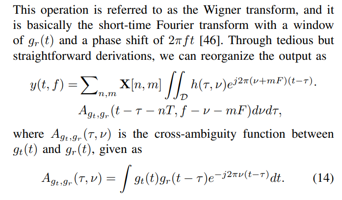
In the previous section, we showed how the D-D domain channel model is related to that in the conventional time-delay domain, and various assumptions in such models are explicitly pointed out. In this section, we will investigate the discrete channel model, laying the foundation for channel interpolation and extrapolation in the next section.
A. Modulation and Demodulation
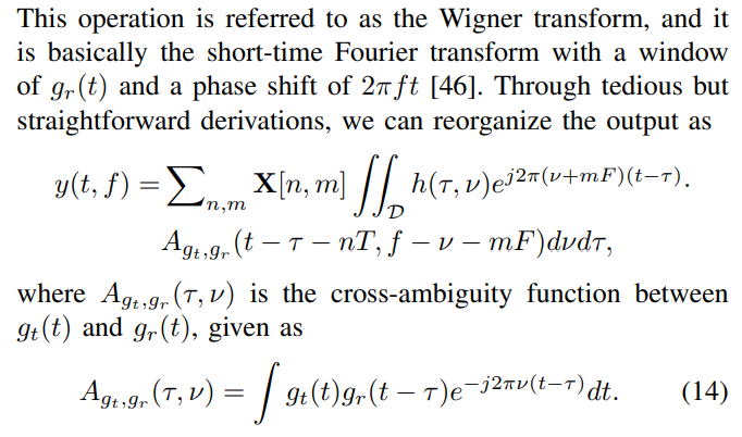

B. Discrete Channel Model
The next step is to discretize the signal in time and frequency domains. Specifically, we sample the 2D signal with an interval of T and F in two dimensions, respectively. The sampled sequence is


B. Discrete Channel Model
The next step is to discretize the signal in time and frequency domains. Specifically, we sample the 2D signal with an interval of T and F in two dimensions, respectively. The sampled sequence is
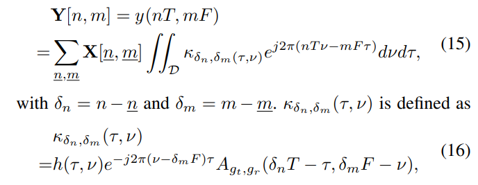

which denotes the impact of a transmitted symbol3 on its neighbours, with a 2D distance of (δn, δm) on the timefrequency grid. From the equations, we can see that the mutual interference among symbols is dependent on both the channel (i.e., system) and the transmitting/receiving pulses (i.e., signal).
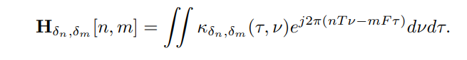
Apart from interference among symbols, another impact of the delay and Doppler spread is channel variation in TF domain, and the channel response at the (n, m)-th T-F slot is


C. Bi-orthogonality
On the right-hand-side of (25), there are two parts. The first part is the desired signal, while the second part is the interference in T-F domain, i.e., ISI and ICI, resulting from the imperfect transmitting/receiving pulses and channel dispersion. Consider OFDM systems with gt(t) and gr(t) being identical rectangular pulses, and Fig. 3 gives the cross-ambiguity function.


In Fig. 3, we can see that the energy of a transmitted symbol will leak to adjacent peers in T-F domain. The red rectangles indicate the delay spread and Doppler spread. With τD = T /10 and νD = F/10, the product of delay and Doppler spread is equal to 0.01. The cross-ambiguity function will exactly attenuate to zero at integer multiples of T and F. For an ideal case with zero delay and Doppler spreads, there will not be ISI and ICI at all, i.e., bi-orthogonality.


The strength of ISI and ICI is dependent on the area of the red rectangle and also the ambiguity function, i.e., (16). This figure gives us an intuitive understanding of how the ISI and ICI are dependent on delay and Doppler spreads. In later discussion, we will refer to the sum of ISI and ICI as ISCI (Inter-SymbolCarrier-Interference).
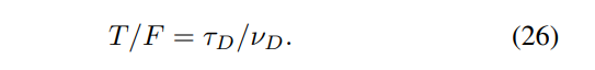
T and F should be chosen carefully to minimize the ISCI. In [45], the authors investigated optimal pulse design, and they showed that the T-F spread of the modulation pulse should be proportional to the channel spread in D-D domain. For rectangular waveforms in particular, we should choose T and F based on

We will follow this rule in the simulations.
:::info
Authors:
(1) Zijun Gong, Member, IEEE;
(2) Fan Jiang, Member, IEEE;
(3) Yuhui Song, Student Member, IEEE;
(4) Cheng Li, Senior Member, IEEE;
(5) Xiaofeng Tao, Senior Member, IEEE.
:::
:::info
This paper is available on arxiv under CC BY-NC-ND 4.0 license.
:::
[2] In general we have T F > 1, and example include CP-OFDM and OFDM with guard intervals. The modeling and algorithm design would be similar.
[3] To be specific, it is a replica of the transmitted symbol delayed by τ and shifted by ν in frequency. The symbol is experiencing spreading due to the multipath effect and Doppler effect. Every replica will have an impact on the received signal, quantified by h(τ, ν).
[4] For N being odd, Diric(N, ω) gives the N-th order Dirichlet kernel.
[5] N × M SFFT is basically N-point IDFT vertically and M-point DFT horizontally. If the size of target matrix is smaller than M × N, it will be zero-padded to M × N.


