


Table of Links
Abstract and 1. Introduction
-
Some recent trends in theoretical ML
2.1 Deep Learning via continuous-time controlled dynamical system
2.2 Probabilistic modeling and inference in DL
2.3 Deep Learning in non-Euclidean spaces
2.4 Physics Informed ML
-
Kuramoto model
3.1 Kuramoto models from the geometric point of view
3.2 Hyperbolic geometry of Kuramoto ensembles
3.3 Kuramoto models with several globally coupled sub-ensembles
-
Kuramoto models on higher-dimensional manifolds
4.1 Non-Abelian Kuramoto models on Lie groups
4.2 Kuramoto models on spheres
4.3 Kuramoto models on spheres with several globally coupled sub-ensembles
4.4 Kuramoto models as gradient flows
4.5 Consensus algorithms on other manifolds
-
Directional statistics and swarms on manifolds for probabilistic modeling and inference on Riemannian manifolds
5.1 Statistical models over circles and tori
5.2 Statistical models over spheres
5.3 Statistical models over hyperbolic spaces
5.4 Statistical models over orthogonal groups, Grassmannians, homogeneous spaces
-
Swarms on manifolds for DL
6.1 Training swarms on manifolds for supervised ML
6.2 Swarms on manifolds and directional statistics in RL
6.3 Swarms on manifolds and directional statistics for unsupervised ML
6.4 Statistical models for the latent space
6.5 Kuramoto models for learning (coupled) actions of Lie groups
6.6 Grassmannian shallow and deep learning
6.7 Ensembles of coupled oscillators in ML: Beyond Kuramoto models
-
Examples
7.1 Wahba’s problem
7.2 Linked robot’s arm (planar rotations)
7.3 Linked robot’s arm (spatial rotations)
7.4 Embedding multilayer complex networks (Learning coupled actions of Lorentz groups)
-
Conclusion and References
6.1 Training swarms on manifolds for supervised ML
6.1.1 Maximum likelihood
The paper [115] discusses two methods for training (reconstruction) the system (1). The first method is essentially standard ML backpropagation. Given the likelihood function q(ϕ) = q(ϕ1, . . . , ϕN ) and the data distribution p(ϕ) = p(ϕ1, . . . , ϕN ), the maximum likelihood for the observed data is obtained by differentiating the log-likelihood function and setting the derivative to zero:


where h·iq(ϕ) stands for the mathematical expectation w.r. to distribution q(ϕ).
Equations (36) can be solved by the (stochastic) gradient descent method. This algorithm requires approximations of the gradient by iterative sampling from the distribution q(ϕ).
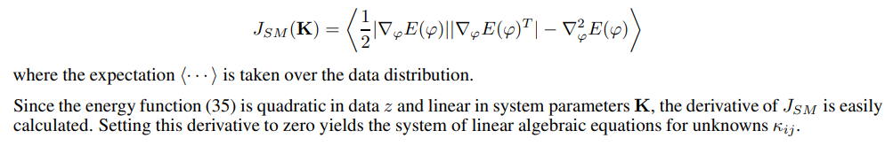
6.1.2 Score matching
An alternative method for training Kuramoto networks is score matching [117]. This method has been implemented in [115] for reconstruction of small networks (consisting of 4-5 oscillators). Introduce the score function:

6.1.3 Evolutionary optimization (CMA ES)
Yet another class of methods for training Kuramoto networks comes from the field of evolutionary optimization and, most notably, the famous CMA ES algorithm [89]. Many experiments demonstrated that CMA ES is competitive with the gradient-based optimization methods when the dimension is not too large (say, the number of parameters is less than one hundred).
Notice, however, that CMA ES performs an update over the Gaussian family and is adapted to Euclidean spaces. This can be suitable for Kuramoto models of the form (1) (the space of Kij is Euclidean, while phase shifts βij are points on the circle). However, when the problem requires learning over the full space of orthogonal matrices, or points on spheres, CMA ES is no longer suitable. In such cases, one can employ evolutionary optimization over manifolds. The stochastic search algorithms over orthogonal groups and spheres can be implemented by performing an update over statistical models considered in the previous Section.
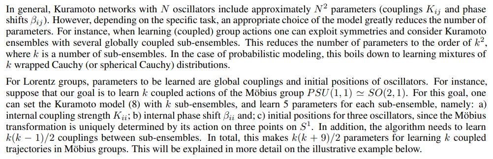
6.1.4 Reduction the number of parameters by choosing an appropriate model

:::info
Author:
(1) Vladimir Jacimovic, Faculty of Natural Sciences and Mathematics, University of Montenegro Cetinjski put bb., 81000 Podgorica Montenegro (vladimirj@ucg.ac.me).
:::
:::info
This paper is available on arxiv under CC by 4.0 Deed (Attribution 4.0 International) license.
:::


