


Table of Links
Abstract and Introduction
Related Work
The media, filter bubbles and echo chambers
Network effects and Information Cascades
Model collapse
Known biases in LLMs
A Model of Knowledge Collapse
Results
Discussion and References
Appendix
Comparing width of the tails
Defining knowledge collapse
Results
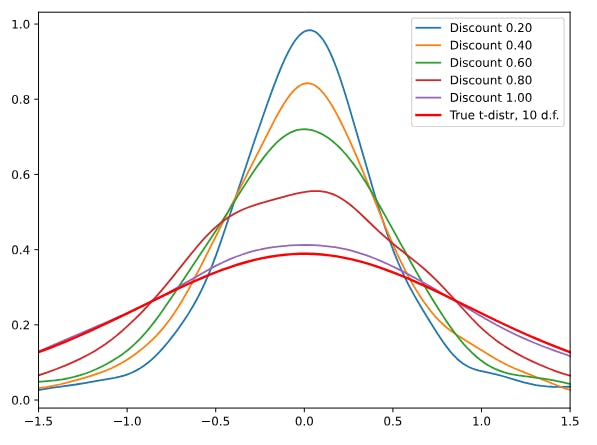
Our main concern is with the view that AI, by reducing the costs of access to certain kinds of information, could only make us better off. In contrast to the literature on model collapse, we consider the conditions under which strategic humans may seek out the input data that will maintain the full distribution of knowledge. Thus, we begin with a consideration of different discount rates. First, we present the a kernel density estimate of public knowledge at the end of 100 rounds (Figure 3). As a baseline, when there is no discount from using AI (discount rate is 1), then as expected public knowledge converges to the true distribution,[9] As AI reduces the cost of truncated knowledge, however, the distribution of public knowledge collapses towards the center, with tail knowledge being under-represented. Under these conditions, excessive reliance on AI-generated content over time leads to a curtailing of the eccentric and rare viewpoints that maintain a comprehensive vision of the world.


Fixing specific parameters, we can get a sense of the size of the the impact of relying on AI. For example, for our default model,[10] after nine generations, when there is no AI discount the public distribution has a Hellinger distance of just 0.09 from the true distribution[11]. When AI-generated content is 20% cheaper (discount rate is 0.8), the distance increases to 0.22, while a 50% discount increases the distance to 0.40. Thus, while the availability of cheap AI-approximations might be thought to only increase public knowledge, under these conditions public knowledge is 2.3 or 3.2 times further away from the truth due to reliance on AI.
For subsequent results illustrating the tradeoff of different parameters, we plot the Hellinger distance between public knowledge at the end of the 100 rounds and the true distribution. First, we examine the importance of updating on the value of relative samples and the relationship to the discount factor in Figure 4. That is, we compare the situation in which individuals do not update on the value of innovation in previous rounds (learning rate near zero, e.g. lr = 0.001) to the case where they update rapidly (here lr = 0.1). As above, the more AI-generated content is cheaper (discount rate indicated by colors), the more public knowledge collapses towards the center. At the same time, when individuals update more slowly on the relative value of learning from AI (the further to the left in the figure), the more public knowledge collapses. We also observe a tradeoff, that is, faster updating on the relative value of AI-generated content can compensate for more extreme price disparities. And conversely, if the discount rate is not too extreme, even slower updating on the relative values is not too harmful.


In Figure 5, we consider the impact of variations in how extreme the truncation of AI-generated content is on the collapse of knowledge. Intuitively, extreme truncation (small values of σtr) correspond to a situation in which AI, for example, summaries an idea with only the most obvious or common perspective. Less extreme truncation corresponds to the idea that AI manages to represent a variety of perspectives, and excludes only extremely rare or arcane perspectives. Naturally, in the latter case, (e.g. if AI truncates the distribution two standard deviations from the mean), the effect is minimal. If AI truncates knowledge outside of 0.25 standard deviations from the mean, the impact is large, though once again this is at least someone moderated when the discount is smaller (especially if there is no generational effect).
We compare the effect of the generational compounding of errors in Figure 6. If there is no generational change, there is at worst only a reduction in the tails of public knowledge outside the truncation limits. In this case the distribution is stable and does not “collapse”, 0.25 0.50 0.75 1.00 1.25 1.50 1.75 2.00 Truncation 0.2 0.3 0.4 0.5 0.6 Hellinger Distance Discount Factor 0.1 0.2 0.3 0.4 0.5 0.6 0.7 0.8 0.9 1.0 Figure 5: Discount rate and truncation limits that is, over time the problem is not progressively worse. We see a jump from this baseline to the case where there is generational change, though the effect of how often generational change occurs (every 3, 5, 10, or 20 rounds) does not have a significant impact.
[9] Even with no discount, there are occasional samples from the truncated distribution, but only enough to realize that they are of relatively less worth than full-distribution samples
[10] Truncation at σtr = 0.75 standard deviations from the mean, generations every 10 rounds, learning rate of 0.05.
[11] Even here there are occasional samples from the truncated distribution – just enough to realize that they have less value than the full-distribution samples.

