The Simple River Measurement That Predicts Ecosystem Collapse | HackerNoon

Table of Links

Abstract and 1. Introduction

2. The well-posed global solution

3. Nontrivial stationary solution

   3.1 Spectral theory of integro-differential operator

   3.2 The existence, uniqueness and stability of nontrivial stationary solution

4. The sharp criteria for persistence or extinction

5. The limiting behaviors of solutions with respect to advection

6. Numerical simulations

7. Discussion, Statements and Declarations, Acknowledgement, and References

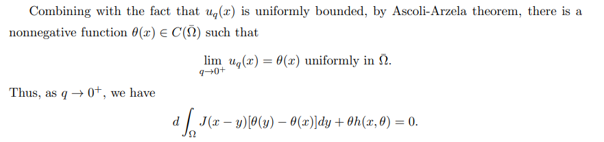
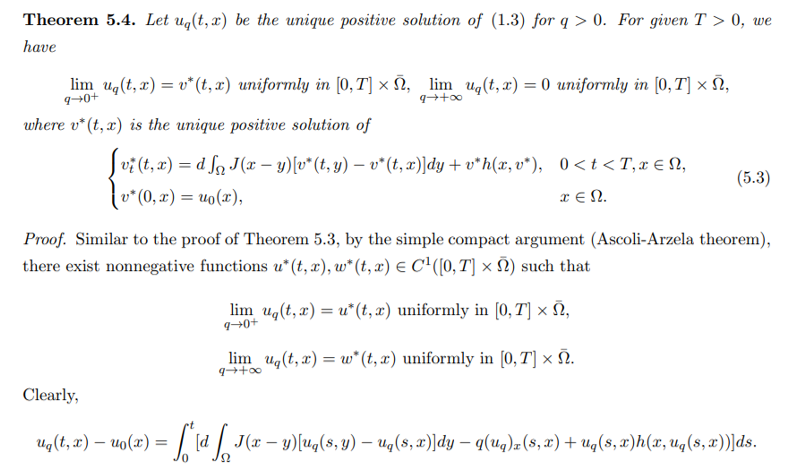
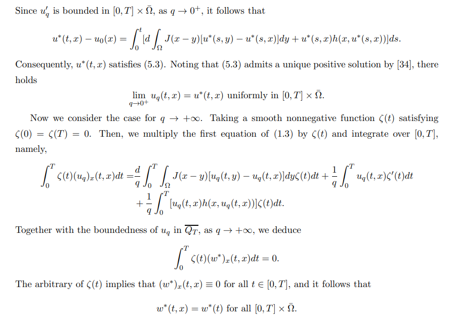
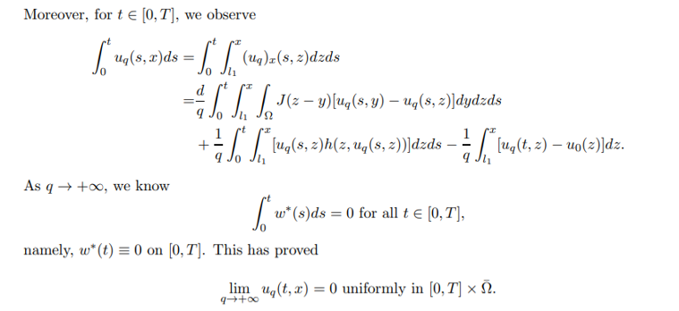
5 The limiting behaviors of solutions with respect to advection

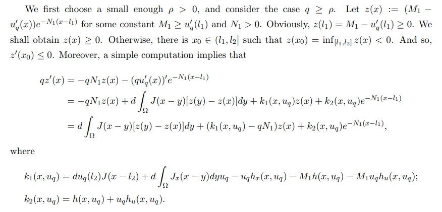
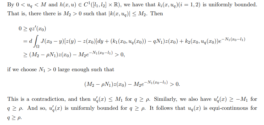
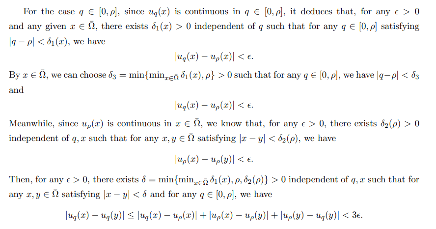
It follows that uq(x) is equi-continuous in q ∈ [0, ρ].

According to [32], the above equation has a unique positive solution for all d > 0.

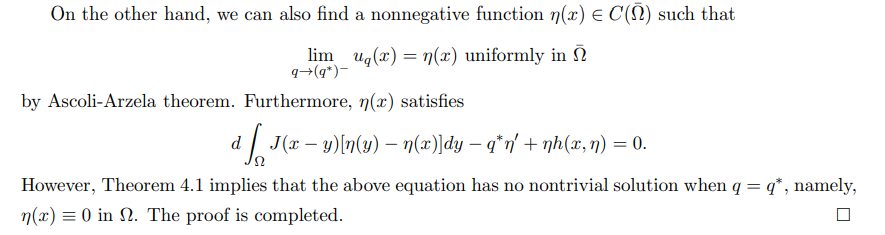
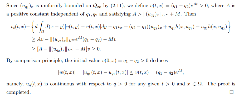
The proof is completed.

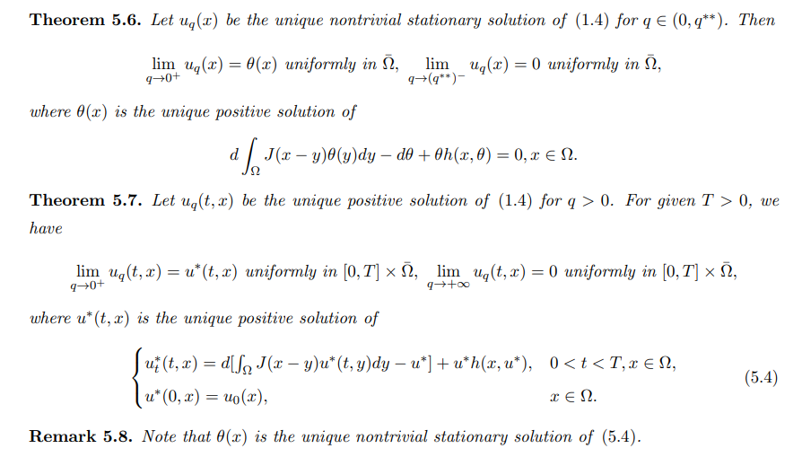
Remark 5.5. Note that γ(x) is the unique nontrivial stationary solution of (5.3).

Similarly, for (1.4), we have

6 Numerical simulations

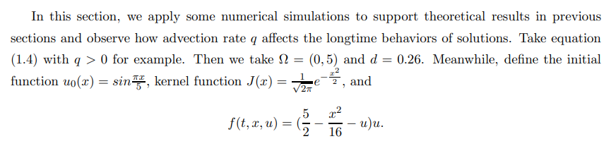
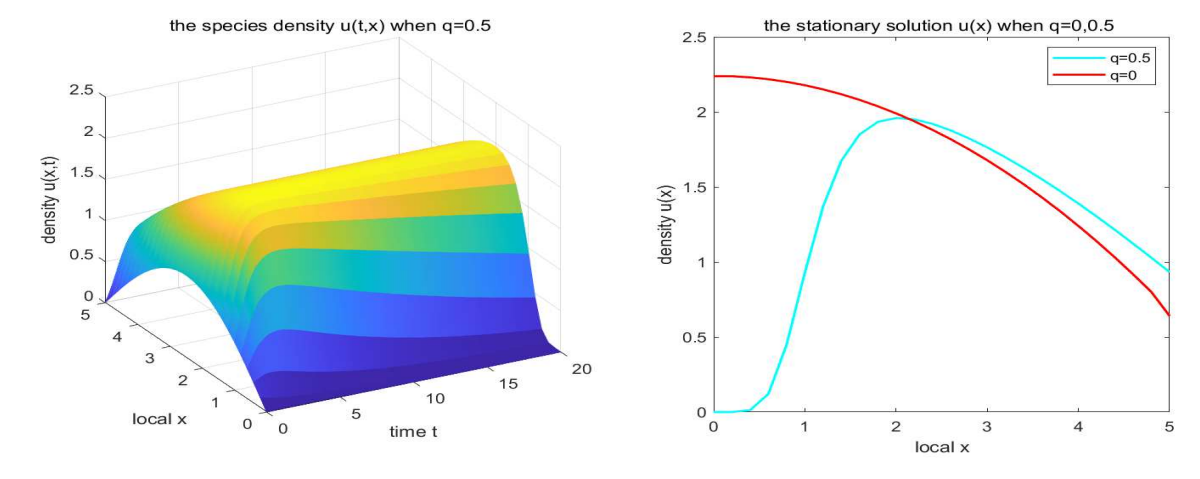
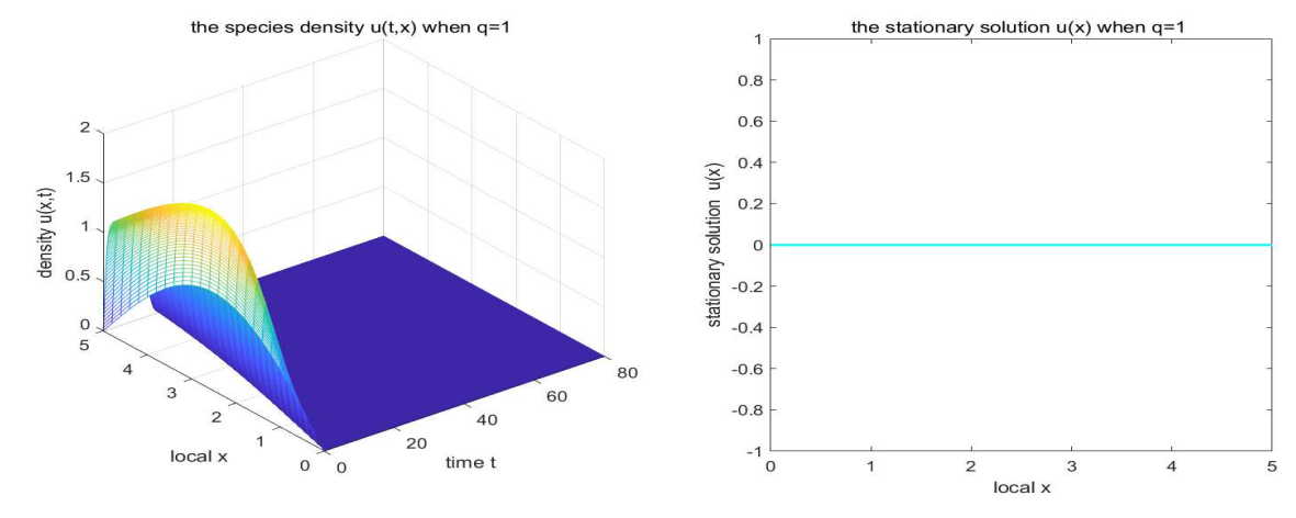
Example 1. A numerical sample for case q = 0.5 is presented in Fig. 1. We observe that species u will ultimately survive and its species density reaches a steady state as time tends to infinite in domain Ω = (0, 5). And from Fig. 1, we find that the advection rate has an impact on the steady state of species density. A numerical sample for case q = 1 is shown in Fig. 2. It follows that species u will extinct in domain Ω = (0, 5), which implies that its species density will tend to 0 as time tends to infinite. Then Figs. 1 and 2 depict the temporal dynamics of species u for system (1.4).

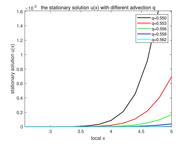
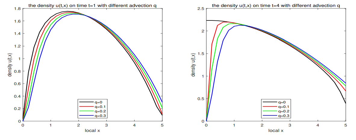
Example 2. Choosing q = 0, 0.1, 0.2, 0.3, by Theorem 4.2, the species will survive and has a steady-state. Figs. 4 and 5 describe the profiles of u with different q at time t = 1, 4 and the profiles of u with different q at location x = 1, 4. We find that when the advection rate has a tendency to 0, the species density will close to the species density for q = 0. Meanwhile, Fig. 6 shows that the stationary solution will close to the stationary solution for q = 0 when the advection rate q tends to 0. These phenomena explain our results for Theorems 5.6 and 5.7 with q → 0 +.

Example 3. By choosing q = 2, 4, 6, 8, we get the profiles of u with different q at time t = 1, 1.2 and the profiles of u with different q at location x = 1, 4; see Figs. 7 and 8. We find that when the advection rate q becomes large, the species density will have a tendency to 0 for any time and location, which explain the result of Theorem 5.7 with q → ∞.

:::info
Authors:

(1) Yaobin Tang, School of Mathematics and Statistics, HNP-LAMA, Central South University, Changsha, Hunan 410083, P. R. China;

(2) Binxiang Dai, School of Mathematics and Statistics, HNP-LAMA, Central South University, Changsha, Hunan 410083, P. R. China (bxdai@csu.edu.cn).

:::

:::info
This paper is available on arxiv under CC BY 4.0 DEED license.

:::