


Authors:
(1) VINÍCIUS YU OKUBO, Dept. Electronic Systems Engineering, Polytechnic School, University of São Paulo, Brazil;
(2) KOTARO SHIMIZU, Department of Applied Physics, The University of Tokyo, Tokyo 113-8656, Japan;
(3) B. S. SHIVARAM, Department of Physics, University of Virginia, Charlottesville, Virginia 22904, USA;
(4) HAE YONG KIM, Dept. Electronic Systems Engineering, Polytechnic School, University of São Paulo, Brazil.
Table of Links
Abstract and I. Introduction
II. Related Work
III. Methodology
IV. Experiments and Results
V. Conclusion and References
A. JUNCTIONS AND TERMINALS DETECTION
Junctions and terminals are shapes with relevance that extend beyond materials. Within computer vision, recognizing and enumerating them has been performed in diverse contexts, such as natural landscapes [20], biology [21] and handwriting images [22].
B. CLASSICAL METHODS FOR JUNCTIONS AND TERMINALS DETECTION
One prevalent approach for detecting junctions and terminals involves using skeletonization as a pre-processing step. This process reduces the image to one-pixel-wide lines to represent its structures. Points in skeleton can then be identified as terminals, junctions and crossings based on their neighboring pixels. This technique has been applied in vascular images [23] and in the analysis of handwritten Chinese characters [24].
Pre-processing techniques using contour information have also been explored for junction detection. Lee and Wu [25] investigated stroke extraction in Chinese characters. Their method segments regions according to their contour, identifying junctions by counting neighboring regions. Maire et al. [26] proposed a junction detector in natural images by locating intersecting contours. This approach applies an expectation–maximization style algorithm to iteratively select relevant contours and suggest the junction’s position.
However, skeletonization and contour finding are noise sensitive processes, and a pre-processing error will lead to a detection error.
Junctions and terminals can also be identified by analyzing the arrangement of linear structures within the image. Su et al. [27] describe a technique for identifying these linear structures using the Hessian Matrix. This approach has been validated in biological images such as blood vessels, neutrites and tree branches. Xia et al. [20] present a junction detection method in natural images, based on amplitudes and phases of the normalized gradients of the image.
Template-based approaches quantify the similarity of the appearance of image regions and the template. Deriche and Blaszka [28] modeled this approach as energy minimization, which is calculated by the deviation between the image and a predetermined model. This enabled the detection of key image features, such as edges, corners and terminals.
C. DEEP LEARNING METHODS FOR JUNCTIONS AND TERMINALS DETECTION
Owing to the success of R-CNN based detection techniques, Pratt et al. [21] developed a pipeline for identifying junctions and crossings in retinal vascular structures. Their method involves two main steps: initially, detection regions are proposed centred along the blood vessels, which are then classified as junctions, crossings or background. To generate the detection regions, their approach requires a binary segmented version of the exam. Theses images undego a skeletonization process, with the resulting points serving as references for the centers of the blood vessels.
Zhao et al. [29], addressing the same problem, proposed using a Mask R-CNN base model [30] for region proposal. This strategy enables inference without the need for binary segmented version of the exam. However, during training, the segmented images are still used in the Mask R-CNN model to enhance its learning capabilities. This approach surpassed the performance of previous techniques in the detection of junctions and crossings in retinal vascular images.
III. METHODOLOGY
A. DATASET
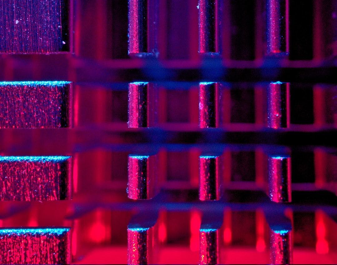
In this study, we used films of a ferromagnetic material of recognized technological importance, Bi:YIG, and obtained magnetic images of the labyrinthine patterns using a microscope with polarized light [31]. We specifically focused on the evolution of the labyrinthine patterns under the demagnetization field protocol described below. First, we prepared the sample in the fully saturated state by applying a sufficiently large magnetic field in +z direction, which is perpendicular to the films. In this state, magnetic moments in the Bi:YIG film are forced to point in the field direction. Next, we instantaneously dropped the field to zero and hold it for 10 seconds to get the image. Since the magnetic field is zero, magnetic moments can point upward and downward, resulting in the labyrinthine patterns shown in Fig. 1; the bright and dark regions represent the domains with opposite directions of magnetic moments. Such a process involving switching on and off the magnetic fields is considered half of the demagnetization step. In the remaining half step, a magnetic field was applied with a reduced amplitude and oriented in the opposite direction. We again captured the magnetic domain image after reducing the magnetic field to zero. By repeating these protocols up to 18 steps, we investigated the evolution of the labyrinthine patterns in the demagnetization process step by step. The amplitude of the magnetic field was exponentially reduced with each step. We conducted a series of demagnetization processes from the fully saturated state, repeating this cycle six times. Furthermore, we explored another situation, where the magnetic field was initially applied in the −z direction, and its direction was alternated step by step. Consequently, a total of 12 demagnetization processes were performed, yielding a collection of 444 domain images. All measurements reported here were performed at room temperature. The experimentally obtained images covered an area of 2 mm × 1.8 mm.
The original high-resolution color images were converted to grayscale and their resolutions were reduced to 1300×972 to facilitate processing. Furthermore, a median filter with kernel size 3 was applied to reduce noise.
B. TM-CNN OVERVIEW
Our approach to detect junctions and terminals in magnetic labyrinthine patterns consists of two sequential steps: proposal of potential detections and their classification between junction, terminal and false detections. It is inspired by other cascaded object detection techniques like Viola and Jones face detection [8], R-CNN [12], and scale and rotation invariant template matching [32].
Fig. 3 illustrates the overall structure of TM-CNN. In the first phase, the algorithm generates a preliminary set of potential detections. It must propose all true defects, even if it also generates many false positives. We achieve this by applying template matching detection with a low threshold, followed by a non-maximum suppression. In the second phase, in order to eliminate the false positives, each potential detection is filtered by a CNN classifier.
C. TEMPLATE MATCHING
The basic form of template matching finds instances of a smaller template T within a larger image I. This is done by calculating some similarity metric between the model T and the content of a moving window located at each possible position of I. We measured the similarity between the image and the template using the Normalized Cross Correlation (NCC). NCC is invariant to linear changes in brightness and/or contrast. NCC between template T and image I at pixel (x, y) is calculated as:


This basic approach is not well suited for detecting junctions and terminals in the magnetic labyrinthine structures because a single template is not capable of modeling:
-
All possible rotations;
-
All deformed shapes of defects.
To solve problem (1), we employ a rotation-invariant template matching based on exhaustive evaluation of rotated templates. There are some alternative rotation-invariant techniques based on circular and radial projections [32], [34], and on Fourier coefficients of circular and radial projections [35]. These techniques can reduce computational requirements, but their implementations are complex and require parameter tuning. Furthermore, our application does not require exceptional computational performance, as the processing is offline. Thus, our technique uses the standard OpenCV[1] template matching implementation, which is highly optimized using FFT and special processor instructions.


D. TEMPLATES AND MASKS USED IN THE EXPERIMENT
We manually designed templates and masks, and empirically tuned them to capture various junction and terminal shapes. They have 21×21 resolutions and are generated at runtime. Templates represent magnetic strips as black lines radiating from their center drawn on a white background. Meanwhile, masks are created from black backgrounds with white areas defining relevant coordinates used in template matching. Their main purpose is to obscure the space between strips and background, addressing variations in widths and curvatures, and to limit the background regions to reduce interference from neighboring strips. Table 1 exemplifies the templates and masks used to detect junctions and terminals.


Template matching is applied separately for each (template, mask) pair. Several template matchings are computed in


parallel using the OpenMP library[2]. This process takes about 80 seconds to process an image on an i7-9750H processor.
To obtain the final correlation map corr, we calculate the maximum value among all n = 3 × 439 + 5 × 120 = 1917 NCC maps for each position (x, y), that is:


Pixels where corr(x, y) exceeds a predefined threshold t are considered potential detections.
However, a single junction/terminal may encompass multiple neighboring points with correlation values greater than the threshold t. Therefore, it is necessary to perform some form of non-maximum suppression to eliminate duplicate detections and select only the true center of junction/terminal. Kim et al. [18] present a solution to this problem: Whenever two potential detection points p1 and p2 are separated by a distance smaller than a threshold c, the point with the lowest correlation value is discarded. In this work, we use a slightly different approach, but with the same practical result: Whenever the algorithm finds a potential detection, it executes a breadth-first search algorithm. This algorithm recursively searches adjacent pixels (x, y) where the correlation exceeds 80% of the threshold (that is, corr(x, y) > 0.8t) and saves the pixel with the highest correlation. Subsequently, the searched area has its correlation value set to zero to avoid re-detection. Fig. 3d highlights the searched area in red. The pixel with the highest correlation is chosen as the center of the junction/termination. This process performs detection in a single pass.
E. DATASET ANNOTATION
To classify potential detections into true or false using a CNN classifier, we must first create annotated training images. TM-CNN makes it easier to create training examples, as it allows one to annotate the examples semi-automatically. This process is divided in two phases.
1) Template matching-assisted annotation
In this phase, only a small set of images are annotated. Initially, we apply template matching followed by nonmaximum suppression to identify the centers of possible detections, together with their probable labels (junction or terminal). Without this help from template matching, we would have to manually and precisely locate the centers of thousands of defects. Subsequently, a human reviewer makes corrections to ensure that the labels given by the template matching are correct. The reviewer may change the labels to junction, terminal or false detection. After all positive detections are annotated along with a small set of false detections, a larger set of false detections is created by lowering the template matching threshold and sampling new false detections. These images, now with positive and negative annotations, are used to train a preliminary version of the CNN classifier.
2) Deep learning-assisted annotation
Due to the small number of images in the initial training set, the preliminary CNN classifier cannot accurately classify all magnetic stripe defects. Nonetheless, this preliminary model is integrated into the annotation procedure to alleviate the required workload. In the second phase, we continue using template matching to generate the initial set of detections. However, the preliminary CNN classifier is employed to identify most of the template matching errors, thus speeding up the annotation process. As new images are annotated, more accurate models are trained to further simplify the annotation workload. The final training set consists of 17 images derived from a single annealing protocol, selected to cover varied experimental configurations of ascending and descending magnetic fields at different magnitudes. Out of these, 16 were selected from the quenched (unordered) state, as they represent a more diverse set of shapes and represent a greater challenge for classification. The training set encompasses a total of 33,772 detections, which includes 12,144 junctions, 12,777 terminals, and 8,851 false detections.
F. CANDIDATE FILTERING BY CNN
Our algorithm extracts small 50×50 patches centered around each detection point and a CNN classifies them into three classes: junction, terminal or false positive. The size of patches for CNN classification is larger than the size of template matching models (21×21), allowing CNN to use more contextual information than template matching.
We use a simple CNN model to classify the small patches (Fig. 4). It has four convolutional layers with 32, 64, 128 and 256 filters, all using 3×3 kernels. The first three convolutional layers are followed by max pooling layers to downsample the feature maps and global max pooling is applied after the last convolutional layer. This is followed by dropout and two fully connected layers: the first with 128 nodes and the second with three output nodes. The ReLU activation function is used across the model, except at the output layer where the softmax is used. In total, this network has only 422,608 parameters. For comparison, VGG-16 and ResNet-50 (common backbones for detection) have 138 million and 23 million parameters, respectively. Thanks to its simplicity, our model is fast and can make predictions even without GPUs and takes around 30 seconds for filtering each image using an i7-9750H processor with 16 GB of RAM.


[1] Open Source Computer Vision Library, https://opencv.org
[2] Open Multi-Processing, https://www.openmp.org/
[3] https://www.tensorflow.org/


