


Understanding how LLMs work in their most fundamental phase helps you understand how they behave and why they behave like that. Building one helps debunk any theory of consciousness in LLMs, but to do so, you would have to choose carefully what text you are training the LLM with— the book “Frankenstein” is the first thought I had in my mind, for some ironic reason.
This tutorial will guide you through all the steps of building an LLM of ~3.2M parameters, solely using Mary Shelley’s Frankenstein. You would not need to run the process on your local computer, as it’s customized to be run on Kaggle Free GPU (God bless Kaggle) in under ~20 minutes if all goes well. You certainly do not need to be a programmer for this, as the code examples would be provided with explanations on syntax as well as the techniques & concepts.
Consider it a complete guide to understand and build an LLM.
(Critical: the LLM we build here would be the rawest of LLMs, as it would not go through stages of fine-tuning/RLHF as commercially available chatbots. It’s merely a model that is not here to help but make predictions and complete your prompts. Refer to Andrej Karparthy’s State of GPT for more. You can find the code here: Buzzpy/Python-Machine-Learning-Models).
Step 1: The Setup & Tokenization
Computers are fundamentally blind to language. They do not look at the word “monster“ and feel a sense of dread or fear. They see signals, which we represent as numbers. The very first step of building an LLM is translating human text into math, through tokenization.
If we were building a public-facing, much larger LLM, we would normally have to go through the process of gathering training data and cleaning it before tokenization. But in our case, since we are only using a book that’s accessible via the Gutenberg Project, we can skip the hard parts and jump into tokenization of the text.
What is Tokenization?
Tokenization is the process of breaking down text into tiny chunks of data (as numbers) that the computer is able to read. A token typically equals 0.75 of a word or roughly 3-4 characters.
Source: Machine Learning Expedition
For this, we are using character-level tokenization; modern, high-parameter-count models (like ChatGPT) use word-level or sub-word level tokenization for efficiency, but in our case, we are focusing our machine to learn English one single letter at a time.
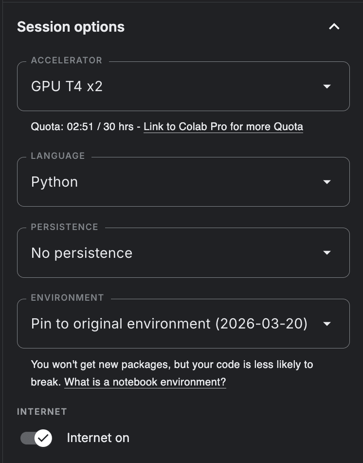
To start, go to Kaggle.com, create a free account, and create your notebook. In the sidebar, make sure the “Internet” toggle is on and “Session options” are set up to run on GPU T4 x 2.

In the notebook, you will note that you can create “blocks“ of code, one already available as an example; this is called a Cell. Replace/create Cell 1 to have this code:
# Importing packages required
import os
import torch
import torch.nn as nn
from torch.nn import functional as F
import urllib.request

# 1. Hardware Setup for Kaggle
os.environ["CUDA_VISIBLE_DEVICES"] = "0"
device="cuda" if torch.cuda.is_available() else 'cpu'

# 2. Hyperparameters (The Architectural Blueprint)
batch_size = 64
block_size = 256
max_iters = 5000
eval_interval = 500
learning_rate = 3e-4
n_embd = 256
n_head = 4
n_layer = 4
dropout = 0.2

torch.manual_seed(1337)

# 3. Downloading the Dataset
print("Downloading Mary Shelley's Frankenstein...")
url = "https://www.gutenberg.org/cache/epub/84/pg84.txt"
req = urllib.request.Request(url, headers={'User-Agent': 'Mozilla/5.0'})
with urllib.request.urlopen(req) as response:
    raw_text = response.read().decode('utf-8')

start_idx = raw_text.find("Letter 1")
end_idx = raw_text.find("*** END OF THE PROJECT GUTENBERG EBOOK")
text = raw_text[start_idx:end_idx] if start_idx != -1 and end_idx != -1 else raw_text

# 4. Tokenization
chars = sorted(list(set(text)))
vocab_size = len(chars)

stoi = { ch:i for i,ch in enumerate(chars) }
itos = { i:ch for i,ch in enumerate(chars) }
encode = lambda s: [stoi[c] for c in s]
decode = lambda l: ''.join([itos[i] for i in l])

# 5. Creating the Tensors
data = torch.tensor(encode(text), dtype=torch.long)
n = int(0.9 * len(data))
train_data = data[:n]
val_data = data[n:]

def get_batch(split):
    data_source = train_data if split == 'train' else val_data
    ix = torch.randint(len(data_source) - block_size, (batch_size,))
    x = torch.stack([data_source[i:i+block_size] for i in ix])
    y = torch.stack([data_source[i+1:i+block_size+1] for i in ix])
    x, y = x.to(device), y.to(device)
    return x, y
The first part of the code (till #2) is about the training setup on Kaggle, not the LLM itself. Note that you will have to edit this setup if you prefer to run the code locally.
Mechanics explained (#2-#5):
-
#2 Hyperparameters: these are the “dials” or controls we use to indicate the size and speed of the model.
-
batch_size = 64: the model will process 64 “chunks“ of text simultaneously.
-
block_size = 256: this is the model’s short-term memory or the “context window“. It can look exactly 256 characters into the past to predict the 257th.
-
n_embed = 256: the number of dimensions in our mathematical space; we are just giving the model a 256-dimensional “room“ to organize concepts/predictions.
-
#3 Downloading: downloads “Frankenstein“ from Project Gutenberg as a TXT file.
-
#4 Tokenization: This is the syntax to split text into characters and tokenize them as discussed before.
-
#5 Tensors: A tensor is a grid of numbers. We convert the entire text of Frankenstein into one massive grid and call it “data“.
-
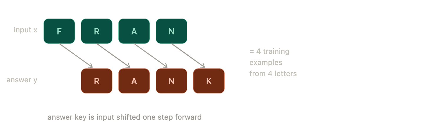
get_batch: The model learns by playing what I (and many, of course) call a game of “guess the next letter”.
The function randomly grabs a chunk of text. Let’s say it grabs a block of 4 letters.
-
The Input (
x): F – R – A – N -
The Answer Key (
y): R – A – N – KNotice that the Answer Key (
y) is the exact same sequence of letters, just shifted forward by one space. The model looks at the Input and makes its guesses, and the Answer Key grades those guesses simultaneously:
-
It looks at F and tries to guess the next letter. The answer key grades it against R.
-
It looks at F – R and tries to guess the next letter. The answer key grades it against A.
… this goes on until the chunk of text is completed.
By shifting the text by one letter, a 256-character blog actually gives the model 256 individual training examples of how letters follow one another.

What the get_batch function does is this splitting of data.
And that’s our Cell 1! We have tokenized the text and set up the boundaries of the LLM.
Step 2: The Core Architecture
Now that we have the main parameters set up, we have to build the actual neural network of the model. Which means that we are building a scaled-down Transformer, the exact same architecture that powers modern AI.
What is a Transformer?
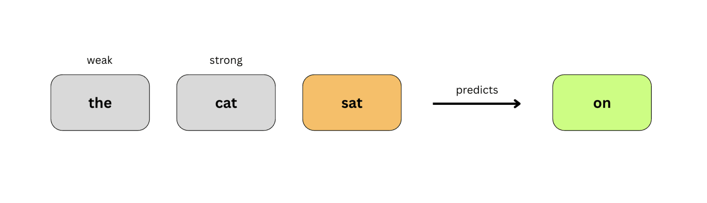
A transformer is yet another machine learning model that is designed to process sequential data in parallel, rather than in order. It look at entire chunks of text all at once, using the mechanism called “Self-attention“. It allows the model to look at a specific word (like “bank“) and instantly scan every other word around it to calculate the context (as in a river or money?).
To do this, create another cell in your Kaggle Notebook (the “+ Code“ button at the end of cell 1 does this) and add this code to it:
# 1. THE ATTENTION HEAD (The "Context" Engine)
class Head(nn.Module):
    def __init__(self, head_size):
        super().__init__()
        self.key = nn.Linear(n_embd, head_size, bias=False)
        self.query = nn.Linear(n_embd, head_size, bias=False)
        self.value = nn.Linear(n_embd, head_size, bias=False)
        self.register_buffer('tril', torch.tril(torch.ones(block_size, block_size)))
        self.dropout = nn.Dropout(dropout)

    def forward(self, x):
        B, T, C = x.shape
        k = self.key(x)
        q = self.query(x)

        # Calculate the mathematical affinities between characters
        wei = q @ k.transpose(-2, -1) * C**-0.5
        # The Mask: Hide the future!
        wei = wei.masked_fill(self.tril[:T, :T] == 0, float('-inf'))
        wei = F.softmax(wei, dim=-1)
        wei = self.dropout(wei)

        v = self.value(x)
        out = wei @ v
        return out

# 2. MULTI-HEAD ATTENTION (Multiple Brains Working Together)
class MultiHeadAttention(nn.Module):
    def __init__(self, num_heads, head_size):
        super().__init__()
        self.heads = nn.ModuleList([Head(head_size) for _ in range(num_heads)])
        self.proj = nn.Linear(n_embd, n_embd)
        self.dropout = nn.Dropout(dropout)

    def forward(self, x):
        out = torch.cat([h(x) for h in self.heads], dim=-1)
        out = self.dropout(self.proj(out))
        return out

# 3. FEED-FORWARD (The "Thinking" Phase)
class FeedForward(nn.Module):
    def __init__(self, n_embd):
        super().__init__()
        self.net = nn.Sequential(
            nn.Linear(n_embd, 4 * n_embd),
            nn.ReLU(),
            nn.Linear(4 * n_embd, n_embd),
            nn.Dropout(dropout),
        )

    def forward(self, x):
        return self.net(x)

# 4. THE TRANSFORMER BLOCK (Putting it Together)
class Block(nn.Module):
    def __init__(self, n_embd, n_head):
        super().__init__()
        head_size = n_embd // n_head
        self.sa = MultiHeadAttention(n_head, head_size)
        self.ffwd = FeedForward(n_embd)
        self.ln1 = nn.LayerNorm(n_embd)
        self.ln2 = nn.LayerNorm(n_embd)

    def forward(self, x):
        x = x + self.sa(self.ln1(x))
        x = x + self.ffwd(self.ln2(x))
        return x

# 5. THE FINAL LLM ASSEMBLY
class EngineeredLLM(nn.Module):
    def __init__(self):
        super().__init__()
        self.token_embedding_table = nn.Embedding(vocab_size, n_embd)
        self.position_embedding_table = nn.Embedding(block_size, n_embd)
        self.blocks = nn.Sequential(*[Block(n_embd, n_head=n_head) for _ in range(n_layer)])
        self.ln_f = nn.LayerNorm(n_embd)
        self.lm_head = nn.Linear(n_embd, vocab_size)

    def forward(self, idx, targets=None):
        B, T = idx.shape
        tok_emb = self.token_embedding_table(idx)
        pos_emb = self.position_embedding_table(torch.arange(T, device=device))
        x = tok_emb + pos_emb
        x = self.blocks(x)
        x = self.ln_f(x)
        logits = self.lm_head(x)

        if targets is None:
            loss = None
        else:
            B, T, C = logits.shape
            logits = logits.view(B*T, C)
            targets = targets.view(B*T)
            loss = F.cross_entropy(logits, targets)
        return logits, loss

    @torch.no_grad()
    def generate(self, idx, max_new_tokens):
        for _ in range(max_new_tokens):
            idx_cond = idx[:, -block_size:]
            logits, _ = self(idx_cond)
            logits = logits[:, -1, :]
            probs = F.softmax(logits, dim=-1)
            idx_next = torch.multinomial(probs, num_samples=1)
            idx = torch.cat((idx, idx_next), dim=1)
        return idx
This sure looks like a mix of random variables and syntax, but the underlying mechanics are fairly simple. Not really, but it’s not overwhelming at least.
Mechanics Explained:
- #1 Attention Head: This is where context is calculated. It asks “What letter am I looking at (Query), “what letters came before me (Key)”, and “what do those letters actually mean (Value)? “
- Notice the Mask (tril). This is crucial. If we didn’t include this, the model would simply look ahead at the answer key to predict the next letter. The mask blinds the model to the future, forcing it to actually learn the statistical patterns of the past.
- #2 Multi-head Attention: Looking at text through just one lens isn’t enough. We run 4 of the above-mentioned Attention Heads in parallel. One head might focus on vowels, another might focus on punctuation, and another on capitalization. They pool their findings together at the end.
- #3 Feed-Forward: Once the attention mechanisms gather the context from the surrounding letters, the Feed-Forward layer acts as the “reasoning” phase. It passes the data through mathematical filters to finalize its guess.
- #4 The Transformer Block: This is simply the packaging. It combines the Attention (Context) and Feed-Forward (Reasoning) into a single, neat block of logic.
- #5 The Final LLM Assembly: This wires everything together. It creates an Embedding Table, which assigns a set of mathematical coordinates to every character. Eventually, this table will learn that vowels cluster together in one part of the mathematical space, while consonants cluster in another. But right now? This brain is completely empty. We have built the engine, but the dials are set to random static.

And that’s our Transformer architecture! A very small version of it, yes, but nevertheless functional. To teach it English, we have to force it to play a guessing game.
Step 3: Backpropagation
It’s rather a fancy word for training the model.
Right now, 3.27 million parameters in our models are completely randomized. For the model to be able to generate any coherent output from what it has learned, we have to train it.
In case you are confused:
When ML engineers talk about dials, weights or parameters, they are often talking about the exact same thing. They are quite literally a massive list of decimes stored in your computer’s RAM.
Imagine a single “neuron“ in our model is trying to decide of the next letter should be “u”. It looks at the current letter (let’s say it’s “q”). The math looks like this:
(Input “q”) × (Weight) = (Prediction “u”)
The Weight is the parameter. It is a number, like 0.842 or -0.113.
If the weight is a high positive number, it means “Yes, strongly connect ‘q’ and ‘u’.” If the weight is a negative number, it means “No, absolutely do not connect ‘q’ and ‘z’.”
When we say the model starts with “random weights,” it means the computer just randomly assigns numbers like 0.34 or -0.91 to all 3.27 million connections. That is why it guesses randomly at first.
Training an AI, as said before, is a game of “Guess the next letter“. The AI makes a guess, checks the actual text to see if it was right, calculates how wrong it was, and then mathematically turns its “dials“ to be slightly less wrong the next time. Interesting.
To train the model, then, you will have to add this code in Cell 3:
# 1. Booting up the Model and Optimizer
model = EngineeredLLM().to(device)
optimizer = torch.optim.AdamW(model.parameters(), lr=learning_rate)

@torch.no_grad()
def estimate_loss():
    out = {}
    model.eval()
    for split in ['train', 'val']:
        losses = torch.zeros(200)
        for k in range(200):
            X, Y = get_batch(split)
            logits, loss = model(X, Y)
            losses[k] = loss.item()
        out[split] = losses.mean()
    model.train()
    return out

print(f"Forging a {sum(p.numel() for p in model.parameters())/1e6:.2f}M parameter model...")

for iter in range(max_iters):
    if iter % eval_interval == 0 or iter == max_iters - 1:
        # 2. Checking the Error Score (Loss)
        losses = estimate_loss()
        print(f"Step {iter}: Train Loss {losses['train']:.4f}, Val Loss {losses['val']:.4f}")

    # 3. Grab a chunk of text and make a guess
    xb, yb = get_batch('train')
    logits, loss = model(xb, yb)

    # 4. Backpropagation (The Calculus)
    optimizer.zero_grad(set_to_none=True)
    loss.backward()

    # 5. Updating the Weights
    optimizer.step()

print("Training complete.")
This part of the code is fairly easy to read and understand; it’s a set of often-used mechanics in LLM training.
Mechanics explained:
- #1 The Optimizer: The optimizer (AdamW) is the algorithm responsible for actually turning the 3.27 million “dials” in the neural network to improve the model’s accuracy.
- #2 Loss: This is the error score, calculated by referencing the original text. A higher loss means it’s guessing blindly (inaccurate), whereas a low loss means it has successfully learned the patterns of English. The earliest loss values will always be higher, as it has not “learned“ at the very beginning.
- #3 Making a guess: We feed the model a chunk of text (xb) and the answer key(yb). It generates its predictions (logits) and compares them to the answer key to calculate the loss as described before.
- #4 Backpropagation (loss.backward()): The fancy word again, but it’s a crucial concept in ML. Once the model knows how wrong it is in a certain guess, it uses calculus to trace that error backward through the entire network, determining exactly which of the 3.27 million dials caused the mistake.
- #5 Updating the Weights: The optimizer takes the information from backpropagation and changes the dials slightly in the correct directions. We do this 6000 times (this allows micro “changes” to dials rather than massive ones). Note that if you change this to some higher number for accuracy, it will backfire, memorizing the book word-for-word, which is called “overfitting“
[When you run this cell, it will take roughly 20 to 30 minutes on the Kaggle GPU. You will see that the Val Loss steadily drops from around 4.6 down to ~1.2. That is the exact threshold where the model suddenly figures out how to construct 19th-century English.]
Now’s a perfect time for a sigh. The training is done.


But if you feel like we went spiraling in the training phase, here is a relatively simple explanation:
- The model takes a chunk of text.
- It pushes that text through the Embedding grids and Linear webs (multiplying the text by the 3.27 million random decimal numbers).
- It spits out a guess for the next letter.
- The Loss function grades the guess.
- Backpropagation uses calculus to figure out exactly which of those 3.27 million decimals were slightly too high, and which were slightly too low.
- The Optimizer (AdamW) goes in and adjusts those decimals by a tiny fraction (e.g., changing a weight from
0.110to0.112).
It repeats this 6,000 times. By the end, those 3.27 million decimals have been perfectly arranged so that when you multiply the letters “I am alon” by those parameters, the math perfectly equals “e”.
Step 4: Inference
Why build a model if you can’t chat with it? Well, actually, you can not “chat“ with the LLM you built in the sense of chatting with ChatGPT or Claude. Because, right now, the model has no instruction or required fine-tuning to make it a helpful assistant who would answer questions like “Why does the creature have no name?”.
But it can absolutely do this: predict. The fundamental ability of all LLMs.
This means that if you feed it a “starting thought“, i.e., an incomplete sentence, it can complete it based on what it has learned. And a raw LLM’s ability to generate any sort of coherent output itself should be praised because it was built with pure math and computing!
To let it speak, add this code to Cell 4 of your Kaggle Notebook:
# 1. Lock the Weights
model.eval()

print("n================================================")
print("      TYPE 'quit' TO EXIT.   ")
print("================================================n")

while True:
    user_input = input("Feed the mirror a starting thought: ")

    if user_input.lower() == 'quit':
        print("Shutting down.")
        break

    # 2. Translate text to numbers
    context_list = encode(user_input)
    context_tensor = torch.tensor([context_list], dtype=torch.long, device=device)

    # 3. Generate the Output
    generated_idx = model.generate(context_tensor, max_new_tokens=500)

    # 4. Translate numbers back to text
    print("n--- The Output ---")
    print(decode(generated_idx[0].tolist()))
    print("----------------n")
This code is just an input-output loop that lets you input a starting thought, and the model will generate an output.
It locks the parameters so the model stops learning, takes the words you typed, convert into integers so the math can process them. It then called the generate function from Cell 2. When the model predicts the next letter, it doesn’t just pick the single highest probability. If it did, it would get stuck repeating “the the the.” Instead, it creates a probability distribution (e.g., “e” is 70% likely, “a” is 20% likely).
Given that the model was trained on Mary Shelley’s Frankenstein, I could not help but use these starting thoughts.
-
Input: “You are my creator, but I am your”
Output: “You are my creator, but I am your miserable forbiddence.”
-
Input: “The greatest tragedy of the human soul is our unending desire to”
Output: “The greatest tragedy of the human soul is our unending desire to made. n Life, although they were explained by the just far as I did not see the…”
-
Input: “My creator gave me a mind, but he forgot to”
Output: “My creator gave me a mind, but he forgot to one, therefore that I n knew that I have no collect.”
If the model’s output were Shelley’s writings verbatim, it has memorized them. If it did not, it has learned from it. And notice the errors! Mostly coherent, mostly not. That is what’s intended when you build an LLM based on a single piece of writing, but based on my experience, this is pretty impressive. It has learned many words and the way to put them together.
A few notes: if your input has spelling mistakes or modern words (say “AI”), the model’s math will be clueless and produce gibberish. Beware.
That is all it is for building your own large language model right from scratch.
You can find the code here: Buzzpy/Python-Machine-Learning-Models


