3 Ways to Easily Visualize Keras Machine Learning Models | HackerNoon

The old cliche “a picture is worth a thousand words” might be even more true when working with complex machine learning models. Unless you are blessed with a photographic memory, you can quickly lose track of the model architecture when just reading through code.

Luckily, there are some easy ways to visualize machine learning models. This guide focuses on the visualization of Keras models and it uses the following model (the “test model”) for demonstration:

def build_model(pad_len, imu_dim, tof_dim, n_classes):
   def time_sum(x):
      return K.sum(x, axis=1)

   def squeeze_last_axis(x):
      return tf.squeeze(x, axis=-1)

   def expand_last_axis(x):
      return tf.expand_dims(x, axis=-1)    
    
   filters_l1 = 64
   kernel_l1 = 3
   filters_l2 = 128
   kernel_l2 = 5
   reduction = 8
   pool_size = 2
   drop = 0.3
   wd = 1e-4
    
   inp = Input(shape=(pad_len, imu_dim + tof_dim))
   imu = Lambda(lambda t: t[:, :, :imu_dim])(inp)
   tof = Lambda(lambda t: t[:, :, imu_dim:])(inp)

   # First CNN branch
   shortcut_1 = imu
   x1 = Conv1D(filters_l1, kernel_l1, padding="same", use_bias=False, kernel_regularizer=l2(wd))(imu)
   x1 = BatchNormalization()(x1)
   x1 = Activation("relu")(x1)
   x1 = Conv1D(filters_l1, kernel_l1, padding="same", use_bias=False, kernel_regularizer=l2(wd))(x1)
   x1 = BatchNormalization()(x1)
   x1 = Activation("relu")(x1)

   ch = x1.shape[-1]
   se = GlobalAveragePooling1D()(x1)
   se = Dense(ch//reduction, activation="relu")(se)
   se = Dense(ch, activation="sigmoid")(se)
   se = Reshape((1, ch))(se)
   x1 = Multiply()([x1, se])

   if shortcut_1.shape[-1] != filters_l1:
      shortcut_1 = Conv1D(filters_l1, 1, padding="same", use_bias=False, kernel_regularizer=l2(wd))(shortcut_1)
      shortcut_1 = BatchNormalization()(shortcut_1)
    
   x1 = add([x1, shortcut_1])
   x1 = Activation("relu")(x1)
   x1 = MaxPooling1D(pool_size)(x1)
   x1 = Dropout(drop)(x1)

   shortcut_2 = x1
   x1 = Conv1D(filters_l2, kernel_l2, padding="same", use_bias=False, kernel_regularizer=l2(wd))(x1)
   x1 = BatchNormalization()(x1)
   x1 = Activation("relu")(x1)
   x1 = Conv1D(filters_l2, kernel_l2, padding="same", use_bias=False, kernel_regularizer=l2(wd))(x1)
   x1 = BatchNormalization()(x1)
   x1 = Activation("relu")(x1)

   ch = x1.shape[-1]
   se = GlobalAveragePooling1D()(x1)
   se = Dense(ch//reduction, activation="relu")(se)
   se = Dense(ch, activation="sigmoid")(se)
   se = Reshape((1, ch))(se)
   x1 = Multiply()([x1, se])

   if shortcut_2.shape[-1] != filters_l2:
      shortcut_2 = Conv1D(filters_l2, 1, padding="same", use_bias=False, kernel_regularizer=l2(wd))(shortcut_2)
      shortcut_2 = BatchNormalization()(shortcut_2)

   x1 = add([x1, shortcut_2])
   x1 = Activation("relu")(x1)
   x1 = MaxPooling1D(pool_size)(x1)
   x1 = Dropout(drop)(x1)
    
   # Second CNN branch
   x2 = Conv1D(filters_l1, kernel_l1, padding="same", use_bias=False, kernel_regularizer=l2(wd))(tof)
   x2 = BatchNormalization()(x2)
   x2 = Activation("relu")(x2)
   x2 = MaxPooling1D(2)(x2)
   x2 = Dropout(0.2)(x2)
   x2 = Conv1D(filters_l2, kernel_l1, padding="same", use_bias=False, kernel_regularizer=l2(wd))(x2)
   x2 = BatchNormalization()(x2)
   x2 = Activation("relu")(x2)
   x2 = MaxPooling1D(2)(x2)
   x2 = Dropout(0.2)(x2)    

   merged = Concatenate()([x1, x2])

   xa = Bidirectional(LSTM(128, return_sequences=True, kernel_regularizer=l2(wd)))(merged)
   xb = Bidirectional(GRU(128, return_sequences=True, kernel_regularizer=l2(wd)))(merged)
   xc = GaussianNoise(0.09)(merged)
   xc = Dense(16, activation="elu")(xc)

   x = Concatenate()([xa, xb, xc])
   x = Dropout(0.4)(x)
   score = Dense(1, activation="tanh")(x)
   score = Lambda(squeeze_last_axis)(score)
   weights = Activation("softmax")(score)
   weights = Lambda(expand_last_axis)(weights)
   context = Multiply()([x, weights])
   x = Lambda(time_sum)(context)

   x = Dense(256, use_bias=False, kernel_regularizer=l2(wd))(x)
   x = BatchNormalization()(x)
   x = Activation("relu")(x)
   x = Dropout(0.5)(x)

   x = Dense(128, use_bias=False, kernel_regularizer=l2(wd))(x)
   x = BatchNormalization()(x)
   x = Activation("relu")(x)
   x = Dropout(0.3)(x)

   out = Dense(n_classes, activation="softmax", kernel_regularizer=l2(wd))(x)
   return Model(inp, out)

As you can see, the model above is reasonably complex. It is used to learn patterns from intertial measurement unit (“IMU”) and other sensor data. To be clear, I didn’t build it. It is referenced from this Kaggle notebook. As you will note, the model definition in the original notebook uses custom objects to encapsulate certain logic that is repeated in the model design. I elected to remove those objects and explicity define the logic “inline” so as to better view the complete structure of the model in my slightly modified implementation.

This guide discusses the following 3 visualization tools:

1. Netron

2. The visualkeras Python package

3. TensorBoard

1. Using Netron to Visualize Your Keras Model

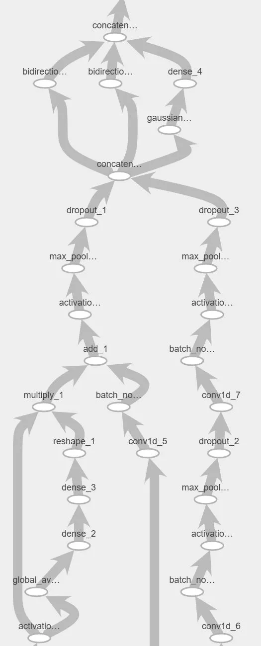
Netron is arguably the simplest visualization tool available. You simply need to click on the Open Model… button on the home page and then select the model that you want to visualize. Here is a visualization of the first few layers of the test model:

Once the model is loaded, you can click on nodes in the model graph to view their properties:

You can export the model graph in .png and .svg formats by clicking on the main menu icon and selecting the appropriate export option.

2. Using visualkeras to Visualize Your Keras Model

The visualkeras Python package is also very easy to use and offers a convenient way to visualize a model before training. You can install the package for your machine learning project using pip:

pip install visualkeras

The following Python code demonstrates basic use of the package:

# [Imports for your Keras model here...]
import visualkeras

# [Utility function to build your Keras model...]
def build_model(model_params):
   # [Your model definition here...]

# [Build the model...]
model = build_model(model_params)

# [Visualize the model...]
visualkeras.graph_view(model).show()

The graph_view method produces the following graphic of the first few layers of the test model:

The package also offers a layered_view method that produces a graphic of the model layers distinguished by type and size:

visualkeras.layered_view(model, legend=True).show()

As seen, passing True to the legend parameter generates a legend describing each layer:

One advantage of the visualkeras package is the control that it offers over how the graphics are displayed. You can review the parameters used to modify the graphic output on the package documentation page.

3. Using TensorBoard to Visualize a Keras Model

TensorBoard is a convenient option for visualization of a Keras model since it is installed along with TensorFlow. With a bit of “massaging”, it is also possible to use TensorBoard to visualize the structure of a model before training.

3.1 Installing the jupyter-tensorboard Package

This section uses TensorBoard within the context of a Jupyter notebook. This requires installation of the jupyter-tensorboard package, which in turn has a couple dependencies. Use the following steps to install jupyter-tensorboard:

1. Install the jupyter package using pip install jupyer.

2. Use the pip install --upgrade notebook==6.4.12 command to downgrade the notebook package which was installed with the jupyter package installation process. The version of the notebook package installed with jupyter which is 7.4.5 as of this writing is not compatible with jupyter-tensorboard. This downgrade step installs a version of the notebook package that is compatible with jupyter-tensorboard. See this StackOverflow article for more information.

3. Install the jupyter-tensorboard package using pip install jupyter-tensorboard.

3.2 Setting Up a Jupyter Notebook to Visualize Your Keras Model

As mentioned above, you can visualize a Keras model in TensorBoard before training it. The following Jupyter notebook code demonstrates how to do it using the test model from the introductory section:

# Cell 1: Imports
import tensorflow as tf
from tensorflow.keras.models import Model, load_model
from tensorflow.keras.layers import (
   Input, Conv1D, BatchNormalization, Activation, add, MaxPooling1D, Dropout,
   Bidirectional, LSTM, GlobalAveragePooling1D, Dense, Multiply, Reshape,
   Lambda, Concatenate, GRU, GaussianNoise
)
from tensorflow.keras.regularizers import l2
from tensorflow.keras import backend as K

# Cell 2: Set logs directory
LOG_DIR = "logs"

# Cell 3: Utility function to build model
# [`build-model` function for test model from introductory section here...]

# Cell 4: Build the model
model = build_model(398, 12, 335, 18)

# Cell 5: Compile the model
model.compile(optimizer="adam", loss="categorical_crossentropy", metrics=["accuracy"])

# Cell 6: Create a TensorBoard callback
tensorboard_callback = tf.keras.callbacks.TensorBoard(
   log_dir=LOG_DIR,
   histogram_freq=1,
   write_graph=True,
   profile_batch=0 # Disable profiling
)

# Cell 7: Create dummy `x` and `y` training inputs that match model input and output shapes
dummy_x_input = tf.random.normal((1, 398, 347)) # Batch size 1, input shape (398,347)
dummy_y_input = tf.random.normal((1, 18)) # Batch size 1, input shape (18, )

# Cell 8: "Train" the model for zero epochs to create a conceptual graph of the model
model.fit(dummy_x_input, dummy_y_input, epochs=0, batch_size=1, callbacks=[tensorboard_callback])

# Cell 9: Load the TensorBoard notebook extension
%load_ext tensorboard

# Cell 10: Launch TensorBoard
%tensorboard --logdir $LOG_DIR --host localhost

If you run the Jupyter notebook code above, the last cell should output Launching TensorBoard. Once the cell execution is complete, you can navigate to http://localhost:6006 to view the TensorBoard dashboard.

3.3 Visualizing Your Keras Model with TensorBoard

TensorBoard should automatically open to the Graphs dashboard. If it doesn’t, you can click on the Graphs menu option or you can alternatively select Graphs from the drop-down menu.

From the Graphs view, select Conceptual graph to view your model’s structure. You should initially see a single node representing the entire model. Double-click on the node to see the sub-graph structure.

You can double-click on individual nodes within the sub-graph structure to view their properties. TensorBoard also allows you to export the model graph in .png format.

Conclusion

Each visualization method discussed above has its pros and cons. Netron is extremely easy to use with trained models whereas visualkeras is arguably the easiest tool to use with untrained models. As seen, TensorBoard can also be used with untrained models, but requires a bit more work to set up properly.