In this article, I intend to try to distill down the essence of diffusion models to give you the basic, core intuition behind them, with code to train a basic diffusion model implemented in PyTorch at the end.
Definition:
🔮 Diffusion model is a type of generative model in Machine Learning, used to generate high-quality data [like images] starting with pure noise. Data is noised through diffusion steps following a Markov chain [as it is a sequence of stochastic events where each time step depends on the previous time step] and then reconstructed by learning the reverse process.
Let us rewind a bit to understand the core idea behind diffusion models. In this paper called “Deep Unsupervised Learning using Non-Equilibrium Thermodynamics”[1], the authors describe it as:
The essential idea, inspired by non-equilibrium statistical physics, is to systematically and slowly destroy structure in a data distribution through an iterative forward diffusion process. We then learn a reverse diffusion process that restores structure in data, yielding a highly flexible and tractable generative model of the data.
The diffusion process essentially is split into a forward and reverse phase. Let us take the example of generating realistic high quality images using diffusion models. The 2 phases would look like this:
-
Forward Diffusion Phase: We start with a real, high-quality image and add noise to it in steps to arrive at pure noise. Basically, we want to destroy the structure in the non-random data distribution that exists at the start.
Here, q is our forward process,
x_t the output of the forward process at time step t,x_(t-1)is an input at time step t. N is a normal distribution withsqrt(1 - β_t) x_{t-1}mean andβ_tIvariance.β_t[also called the schedule] here controls the amount of noise added at time step = t whose value ranges from 0→1. Depending on the type of schedule you use, you arrive at what is close to pure noise sooner or later. i.e. β_1,…,β_T is a variance schedule (that is either learned or fixed) which, if well-behaved, ensures thatx_Tis almost an isotropic Gaussian at sufficiently large T. -
Reverse Diffusion Phase: This is where the actual machine learning takes place. As the name suggests, we try to transform the noise back into a sample from the target distribution in this phase. i.e. the model is learning to denoise pure Gaussian noise into a clean image. Once the neural network has been trained, this ability can be used to generate new images out of Gaussian noise through step-by-step reverse diffusion.
Since one cannot readily estimate
q(x_(t-1)|x_t), we need to learn a modelp_thetato approximate the conditional probabilities for the reverse diffusion process. -
We want to model the probability density of an earlier time step given the current. If we apply this reverse formula for all time steps T→0, we can trace our steps back to the original data distribution. The time step information is provided usually as positional embeddings to the model. It is worth mentioning here that the diffusion model predicts the entire noise to be removed at a given timestep to make it equivalent to the image at the start, and not just the delta between the current and previous time step. However, we only subtract part of it and move to the next step. That is how the diffusion process works.


To summarize, fundamentally, a diffusion model destroys the structure in training data through the successive addition of Gaussian noise, and then learns to recover what it broke by reversing this noising process. After training, one can use the diffusion model to generate data by simply passing randomly sampled noise through the “learned” denoising process. For a detailed mathematical explanation, check out this blog [4].
Implementation:
We shall use the Oxford Flowers102 dataset, which contains images of flowers across 102 categories, and build a very simple model for the purposes of this article to understand the core idea and implementation of diffusion models. Repository [5] serves as a great reference.
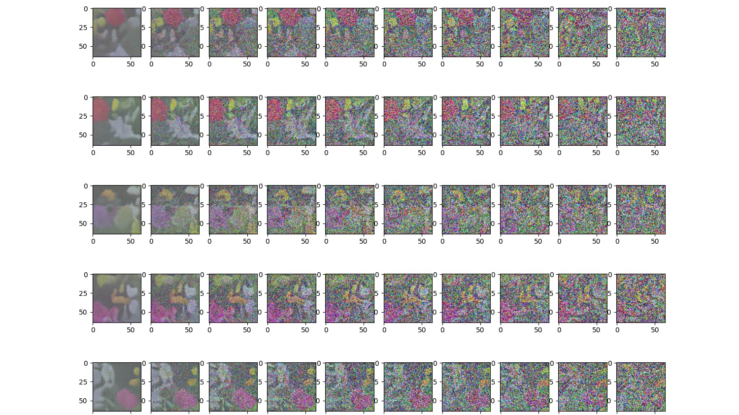
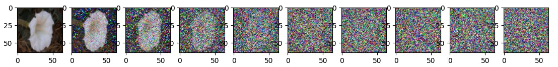
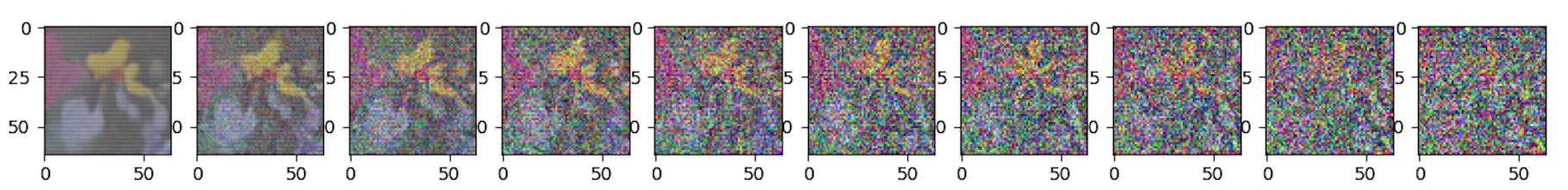
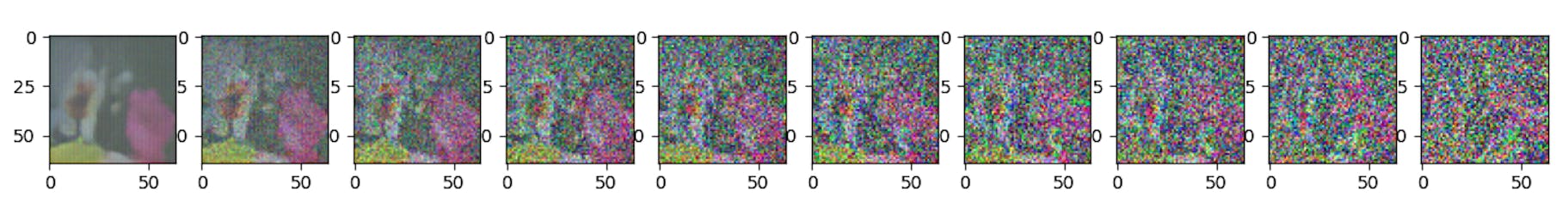
Forward phase: Since the sum of Gaussians is also a Gaussian, though the noise addition is sequential, one can pre-compute a noisy version of the input image for a specific time step [2]. This follows Equation 4 from [2]
def linear_beta_schedule(timesteps, start=1e-4, end=2e-2):
    """Creates a linearly increasing noise schedule."""
    return torch.linspace(start, end, timesteps)

def get_idx_from_list(vals, t, x_shape):
    """ Returns a specific index t of a passed list of values vals. """
    batch_size = t.shape[0]
    out = vals.gather(-1, t.cpu())
    return out.reshape(batch_size, *((1,) * (len(x_shape) - 1))).to(t.device)

def forward_diffusion_sample(x_0, t, device="cpu"):
    """ Takes an image and a timestep as input and returns the noisy version of it."""
    noise = torch.randn_like(x_0)
    sqrt_alphas_cumprod_t = get_index_from_list(sqrt_alphas_cumprod, t, x_0.shape)
    sqrt_one_minus_alphas_cumprod_t = get_idx_from_list(sqrt_one_minus_alphas_cumprod, t, x_0.shape)
    return sqrt_alphas_cumprod_t.to(device) * x_0.to(device) + sqrt_one_minus_alphas_cumprod_t.to(device) * noise.to(device), noise.to(device)


T = 300  # Total number of timesteps
betas = linear_beta_schedule(T)
# Precompute values for efficiency
alphas = 1. - betas
alphas_cumprod = torch.cumprod(alphas, dim=0)
alphas_cumprod_prev = F.pad(alphas_cumprod[:-1], (1, 0), value=1.0)

sqrt_recip_alphas = torch.sqrt(1. / alphas)
sqrt_alphas_cumprod = torch.sqrt(alphas_cumprod)
sqrt_one_minus_alphas_cumprod = torch.sqrt(1. - alphas_cumprod)
posterior_variance = betas * (1. - alphas_cumprod_prev) / (1. - alphas_cumprod)
Reverse Diffusion Phase: This is the denoising phase where the model learns to estimate the noise that was added at each time step. We use a simple U-Net neural network that takes in noisy image and time step [provided as positional embedding] and predicts the noise. Each ConvBlock layer below uses the sinusoidal time step embedding, capturing temporal context to condition the convolutional output. This architecture is inspired by [2] and optimized variants presented in [3].
class SinusoidalPositionEmbeddings(nn.Module):
    def __init__(self, dim):
        super().__init__()
        self.dim = dim

    def forward(self, t):
        half_dim = self.dim // 2
        scale = math.log(10000) / (half_dim - 1)
        freqs = torch.exp(torch.arange(half_dim, device=t.device) * -scale)
        angles = t[:, None] * freqs[None, :]
        return torch.cat([angles.sin(), angles.cos()], dim=-1)

class ConvBlock(nn.Module):
    def __init__(self, in_channels, out_channels, time_emb_dim, upsample=False):
        super().__init__()
        self.time_mlp = nn.Linear(time_emb_dim, out_channels)
        self.upsample = upsample

        self.conv1 = nn.Conv2d(in_channels * 2 if upsample else in_channels, out_channels, kernel_size=3, padding=1)
        self.transform = (
            nn.ConvTranspose2d(out_channels, out_channels, kernel_size=4, stride=2, padding=1)
            if upsample else
            nn.Conv2d(out_channels, out_channels, kernel_size=4, stride=2, padding=1)
        )
        self.conv2 = nn.Conv2d(out_channels, out_channels, kernel_size=3, padding=1)
        self.bn1 = nn.BatchNorm2d(out_channels)
        self.bn2 = nn.BatchNorm2d(out_channels)
        self.relu = nn.ReLU()

    def forward(self, x, t):
        h = self.bn1(self.relu(self.conv1(x)))
        time_emb = self.relu(self.time_mlp(t))[(..., ) + (None,) * 2]
        h = h + time_emb
        h = self.bn2(self.relu(self.conv2(h)))
        return self.transform(h)

class SimpleUNet(nn.Module):
    """Simplified U-Net for denoising diffusion models."""

    def __init__(self):
        super().__init__()
        image_channels = 3
        down_channels = (64, 128, 256, 512, 1024)
        up_channels = (1024, 512, 256, 128, 64)
        output_channels = 3
        time_emb_dim = 32

        self.time_mlp = nn.Sequential(
            SinusoidalPositionEmbeddings(time_emb_dim),
            nn.Linear(time_emb_dim, time_emb_dim),
            nn.ReLU()
        )
        self.init_conv = nn.Conv2d(image_channels, down_channels[0], kernel_size=3, padding=1)

        self.down_blocks = nn.ModuleList([
            ConvBlock(down_channels[i], down_channels[i+1], time_emb_dim)
            for i in range(len(down_channels) - 1)
        ])

        self.up_blocks = nn.ModuleList([
            ConvBlock(up_channels[i], up_channels[i+1], time_emb_dim, upsample=True)
            for i in range(len(up_channels) - 1)
        ])

        self.final_conv = nn.Conv2d(up_channels[-1], output_channels, kernel_size=1)

    def forward(self, x, t):
        t_emb = self.time_mlp(t)
        x = self.init_conv(x)
        skip_connections = []

        for block in self.down_blocks:
            x = block(x, t_emb)
            skip_connections.append(x)

        for block in self.up_blocks:
            skip_x = skip_connections.pop()
            x = torch.cat([x, skip_x], dim=1)
            x = block(x, t_emb)
        return self.final_conv(x)

model = SimpleUnet()
The training objective is a simple MSE loss, computing the difference between the actual noise and the model’s prediction of that noise.
def get_loss(model, x_0, t, device):
    x_noisy, noise = forward_diffusion_sample(x_0, t, device)
    noise_pred = model(x_noisy, t)
    return F.mse_loss(noise, noise_pred)
Finally, after training the model for 300 epochs, we can start generating ~ realistic-looking images of flowers by sampling pure Gaussian noise and feeding it through the learned reverse diffusion process. Below are a few samples I was able to generate this way. It would be worth experimenting with some variations of the above architecture, learning rate, scheduler, and the number of epochs for training.


References:
- Deep Unsupervised Learning using Nonequilibrium Thermodynamics Sohl-Dickstein, J. et al.[2015]
- Denoising Diffusion Probabilistic Models Ho et al. [2020]
- Diffusion Models Beat GANs on Image Synthesis Dhariwal and Nichol [2021]
- This amazing blog for a deeper dive into the math behind diffusion models.
- This repository access to a collection of resources and papers on Diffusion Models.


