By using this site, you agree to the Privacy Policy and Terms of Use.
Accept
World of SoftwareWorld of SoftwareWorld of Software
  • News
  • Software
  • Mobile
  • Computing
  • Gaming
  • Videos
  • More
    • Gadget
    • Web Stories
    • Trending
    • Press Release
Search
  • Privacy
  • Terms
  • Advertise
  • Contact
Copyright © All Rights Reserved. World of Software.
Reading: A Close Look at Misalignment in Pretraining Datasets | HackerNoon
Share
Sign In
Notification Show More
Font ResizerAa
World of SoftwareWorld of Software
Font ResizerAa
  • Software
  • Mobile
  • Computing
  • Gadget
  • Gaming
  • Videos
Search
  • News
  • Software
  • Mobile
  • Computing
  • Gaming
  • Videos
  • More
    • Gadget
    • Web Stories
    • Trending
    • Press Release
Have an existing account? Sign In
Follow US
  • Privacy
  • Terms
  • Advertise
  • Contact
Copyright © All Rights Reserved. World of Software.
World of Software > Computing > A Close Look at Misalignment in Pretraining Datasets | HackerNoon
Computing

A Close Look at Misalignment in Pretraining Datasets | HackerNoon

News Room
Last updated: 2025/07/10 at 8:27 AM
News Room Published 10 July 2025
Share
SHARE

Table of Links

Abstract and 1. Introduction

2 Concepts in Pretraining Data and Quantifying Frequency

3 Comparing Pretraining Frequency & “Zero-Shot” Performance and 3.1 Experimental Setup

3.2 Result: Pretraining Frequency is Predictive of “Zero-Shot” Performance

4 Stress-Testing the Concept Frequency-Performance Scaling Trend and 4.1 Controlling for Similar Samples in Pretraining and Downstream Data

4.2 Testing Generalization to Purely Synthetic Concept and Data Distributions

5 Additional Insights from Pretraining Concept Frequencies

6 Testing the Tail: Let It Wag!

7 Related Work

8 Conclusions and Open Problems, Acknowledgements, and References

Part I

Appendix

A. Concept Frequency is Predictive of Performance Across Prompting Strategies

B. Concept Frequency is Predictive of Performance Across Retrieval Metrics

C. Concept Frequency is Predictive of Performance for T2I Models

D. Concept Frequency is Predictive of Performance across Concepts only from Image and Text Domains

E. Experimental Details

F. Why and How Do We Use RAM++?

G. Details about Misalignment Degree Results

H. T2I Models: Evaluation

I. Classification Results: Let It Wag!

F Why and How Do We Use RAM++?

We detail why we use the RAM++ model [59] instead of CLIPScore [56] or open-vocabulary detection models [80]. Furthermore, we elaborate on how we selected the threshold hyperparameter used for identifying concepts in images.

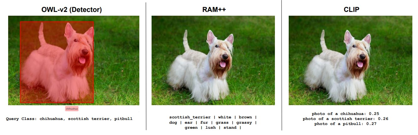
F.1 Why RAM++ and not CLIP or open-vocabulary detectors?

We provide some qualitative examples to illustrate why we chose RAM++. Our input images do not often involve complex scenes suitable for object detectors, but many fine-grained classes on which alongside CLIP, even powerful open-world detectors like OWL-v2 [80] have poor performance.

Figure 19: Qualitative Results comparing OWL-v2, RAM++ and CLIP. We show qualitative examples across three different models: OWL-v2, RAM++ and CLIP on fine-grained concepts.Figure 19: Qualitative Results comparing OWL-v2, RAM++ and CLIP. We show qualitative examples across three different models: OWL-v2, RAM++ and CLIP on fine-grained concepts.

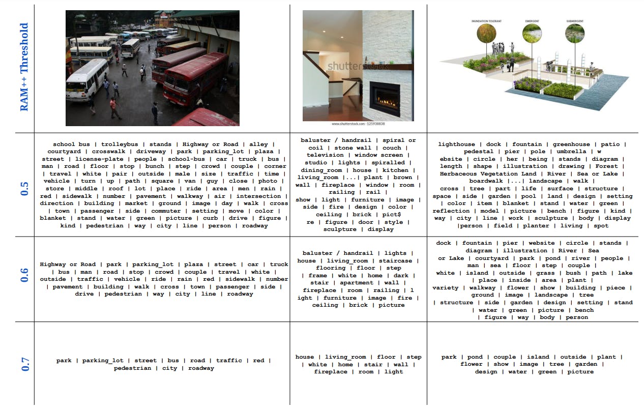
F.2 How: Optimal RAM++ threshold for calculating concept frequencies

We ablate the choice of the threshold we use for assigning concepts to images using the RAM++ model. For the given set of concepts, RAM++ provides a probability value (by taking a sigmoid over raw logits) for each concept’s existence in a particular image. To tag an image as containing a particular concept, we have to set a threshold deciding this assignnment. We test over three thresholds: {0.5, 0.6, 0.7}, showcasing quantitative and qualitative results for all thresholds in Figs. 20 and 21.

We observe best frequency estimation results using the highest frequency of 0.7. This is due to the high precision afforded by this threshold, leading to us counting only the “most aligned images” per concept as hits. With lower thresholds (0.5, 0.6), we note that noisier images that do not align well with the concept can be counted as hits, leading to degraded precision and thereby poorer frequency estimation. Hence, we use 0.7 as the threshold for all our main results.

Figure 20: Qualitative Results with different RAM++ thresholds. We show qualitative examples across three different thresholds: {0.5, 0.6, 0.7} for estimating concept frequency using the RAM++ model. We note that the significantly better concepts identified by the higher threshold (0.7) compared to the lower thresholds (0.5, 0.7). The images are sourced from the CC-3M dataset.Figure 20: Qualitative Results with different RAM++ thresholds. We show qualitative examples across three different thresholds: {0.5, 0.6, 0.7} for estimating concept frequency using the RAM++ model. We note that the significantly better concepts identified by the higher threshold (0.7) compared to the lower thresholds (0.5, 0.7). The images are sourced from the CC-3M dataset.

Figure 21: Effect of different thresholds for determining concept frequency using RAM++. We test three different thresholds: {0.5, 0.6, 0.7} for estimating concept frequency using the RAM++ model. We note that the correlations are significantly stronger with a threshold of 0.7—this is justified by the higher precision of image sample hits at a higher threshold (0.7). Comparatively, lower thresholds (0.5, 0.7) lead to noisier images being counted as hits, hence reducing the hit precision for determining frequency. ** indicates that the result is significant (p < 0.05 with two-tailed t-test.), and thus we show pearson correlation (ρ) too.Figure 21: Effect of different thresholds for determining concept frequency using RAM++. We test three different thresholds: {0.5, 0.6, 0.7} for estimating concept frequency using the RAM++ model. We note that the correlations are significantly stronger with a threshold of 0.7—this is justified by the higher precision of image sample hits at a higher threshold (0.7). Comparatively, lower thresholds (0.5, 0.7) lead to noisier images being counted as hits, hence reducing the hit precision for determining frequency. ** indicates that the result is significant (p < 0.05 with two-tailed t-test.), and thus we show pearson correlation (ρ) too.

G Details about Misalignment Degree Results

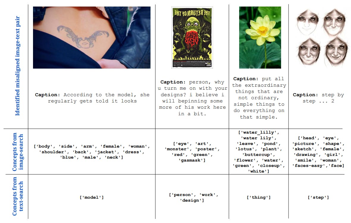
In Tab. 3 in the main paper, we quantified the misalignment degree, and showcased that a large number of image-text pairs in all pretraining datasets are misaligned. In Alg. 1, we describe the method used for quantifying the misalignment degree for each pretraining dataset. We also showcase some qualitative examples of a few image-text pairs from the CC-3M dataset that are identified as misaligned using our analysis.

Algorithm 1: Extracting misalignment degree from pretraining datasetsAlgorithm 1: Extracting misalignment degree from pretraining datasets

Figure 22: Qualitative examples of misaligned image-text pairs identified. We present 4 samples from the CC3M pretraining dataset that are identified as misaligned by our analysis. Here, the text captions clearly do not entail the images, and hence do not provide a meaningful signal for learning.Figure 22: Qualitative examples of misaligned image-text pairs identified. We present 4 samples from the CC3M pretraining dataset that are identified as misaligned by our analysis. Here, the text captions clearly do not entail the images, and hence do not provide a meaningful signal for learning.

Authors:

(1) Vishaal Udandarao, Tubingen AI Center, University of Tubingen, University of Cambridge, and equal contribution;

(2) Ameya Prabhu, Tubingen AI Center, University of Tubingen, University of Oxford, and equal contribution;

(3) Adhiraj Ghosh, Tubingen AI Center, University of Tubingen;

(4) Yash Sharma, Tubingen AI Center, University of Tubingen;

(5) Philip H.S. Torr, University of Oxford;

(6) Adel Bibi, University of Oxford;

(7) Samuel Albanie, University of Cambridge and equal advising, order decided by a coin flip;

(8) Matthias Bethge, Tubingen AI Center, University of Tubingen and equal advising, order decided by a coin flip.


Sign Up For Daily Newsletter

Be keep up! Get the latest breaking news delivered straight to your inbox.
By signing up, you agree to our Terms of Use and acknowledge the data practices in our Privacy Policy. You may unsubscribe at any time.
Share This Article
Facebook Twitter Email Print
Share
What do you think?
Love0
Sad0
Happy0
Sleepy0
Angry0
Dead0
Wink0
Previous Article Keep your pool spotless with the biggest WYBOT sale ever: Save up to $1,000!
Next Article ChatGPT hardware confirmed, as OpenAI closes $6.5B deal for Jony Ive’s startup
Leave a comment

Leave a Reply Cancel reply

Your email address will not be published. Required fields are marked *

Stay Connected

248.1k Like
69.1k Follow
134k Pin
54.3k Follow

Latest News

First NIO-partnered EV with swappable batteries to go on sale in Q3: report · TechNode
Computing
Murderbot is getting a season 2 on Apple TV Plus
News
UK growth appetite is strong as tech firms expect M&A surge – UKTN
News
Outlook outage takes down Microsoft email service for hours
News

You Might also Like

Computing

First NIO-partnered EV with swappable batteries to go on sale in Q3: report · TechNode

1 Min Read
Computing

We Must Stop Bill Essayli Before It’s Too Late – Knock LA

6 Min Read
Computing

Delve into AI: A brand new column about AI in Africa

4 Min Read
Computing

Can You Trust What AI Tells You About PPC? We Tested It! | WordStream

21 Min Read
//

World of Software is your one-stop website for the latest tech news and updates, follow us now to get the news that matters to you.

Quick Link

  • Privacy Policy
  • Terms of use
  • Advertise
  • Contact

Topics

  • Computing
  • Software
  • Press Release
  • Trending

Sign Up for Our Newsletter

Subscribe to our newsletter to get our newest articles instantly!

World of SoftwareWorld of Software
Follow US
Copyright © All Rights Reserved. World of Software.
Welcome Back!

Sign in to your account

Lost your password?