A Simple, Transparent Model for Estimating Ethereum Transaction Speeds | HackerNoon

Table of Links

Abstract and 1 Introduction

2 Background and 2.1 Blockchain

2.2 Transactions

3 Motivating Example

4 Computing Transaction Processing Times

5 Data Collection and 5.1 Data Sources

5.2 Approach

6 Results

6.1 RQ1: How long does it take to process a transaction in Ethereum?

6.2 RQ2: How accurate are the estimates for transaction processing time provided by Etherscan and EthGasStation?

7 Can a simpler model be derived? A post-hoc study

8 Implications

8.1 How about end-users?

9 Related Work

10 Threats to Validity

11 Conclusion, Disclaimer, and References

A. COMPUTING TRANSACTION PROCESSING TIMES

A.1 Pending timestamp

A.2 Processed timestamp

B. RQ1: GAS PRICE DISTRIBUTION FOR EACH GAS PRICE CATEGORY

B.1 Sensitivity Analysis on Block Lookback

C. RQ2: SUMMARY OF ACCURACY STATISTICS FOR THE PREDICTION MODELS

D. POST-HOC STUDY: SUMMARY OF ACCURACY STATISTICS FOR THE PREDICTION MODELS

7 CAN A SIMPLER MODEL BE DERIVED? A POST-HOC STUDY

Motivation. In RQ2, we observed that Etherscan Gas Tracker webpage is the most accurate model for predicting the processing times of very cheap and cheap transactions. However, as of the time this paper was written, Etherscan does not provide any public documentation concerning the design of this model nor how it operates (e.g., the learner being used, the features being used by the model, the model retraining frequency). It is also unclear whether the design of the model has changed since its introduction. We consider that it is undesirable and possibly risky for ÐApp developers to have to rely on an estimation service that lacks transparency [15]. Moreover, we observed in RQ2 that the EthGasStation Gas Price API is the most accurate model for the other gas price categories. Hence, maximizing prediction accuracy across gas price categories implies using two models that are provided by different online estimation services. This setting is likely to induce a higher development and maintenance overhead compared to the possibility of relying on a single, inherently interpretable model.

Therefore, in this post-hoc study, we assess our ability to derive an estimator that is simple, inherently interpretable, and yet performs as accurately as a combination of the Etherscan Gas Tracker webpage and the EthGasStation Gas Price API (hereafter called the state-of-the-practice model).

Approach. In the following, we describe the design and assessment of our model. We organize this description into the following items (a) choice of prediction algorithm, (b) feature engineering, (c) data preprocessing, (d) model validation, (e) accuracy comparison,

a) Choice of prediction algorithm. We choose a linear regression (ordinary least squares) because it is an inherently interpretable model (e.g., as opposed to black box models) [31]. More specifically, a linear regression model predicts the dependent variable as a weighted sum of the independent variables (features) [23]. Since there is a clear mathematical explanation for the predicted value of each observation, linear regressions are deemed as inherently interpretable models. We use the rms R package[16].

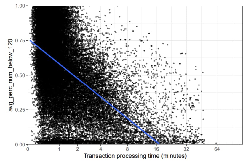
b) Feature engineering and model specification. We engineer only one feature which combines recent contextual and historical information of the Ethereum blockchain. Namely, we define this feature as: the average of the percentage of transactions with gas prices lower than the current transaction in the previous 120 blocks.

Our rationale for implementing this feature is that history-based features have yielded positive results in prediction models throughout several software engineering studies [20, 32, 47]. We believe that historical features can also be leveraged in our context. More specifically, we expect that the dynamics of transaction processing are likely to be similar to those of half an hour ago. For instance, if the network was not clogged half an hour ago, we expect that it will remain unclogged in the vast majority of cases. In light of this rationale, we designed the moving average of the percentage of transactions with gas prices lower than the current transaction in the previous 120 blocks feature. For any given transaction 𝑡, we take the previous 120 blocks (which cover a timespan of 30 minutes on average) and for each of them calculate the percentage of transactions with gas prices less than 𝑡, and finally take the average of these percentages. This feature reflects how competitive the gas price for 𝑡 is, hence if the resulting average percentage is high, the processing time should be fairly quick, and vice versa.

Next, we investigate the relationship between our engineered feature and the processing times of transactions to ensure our models will have adequate explanatory power of processing times. Figure 7 illustrates a negative relationship between the two distributions – as our independent feature increases, processing times decrease, and vice versa. To confirm this we also compute the Spearman’s correlation (𝜌) to analyze the correlation between these two variables. We use Spearman’s correlation in lieu of Person’s correlation because the latter only assesses linear relationships. Spearman’s correlation, in turn, assesses monotonic relationships (linear or not) and is thus more flexible. We assess Spearman’s correlation coefficient using the following thresholds [18], which operate on 2 decimal places only: very weak for |𝜌| ≤ 0.19, weak for 0.20 ≤ |𝜌| ≤ 0.39, moderate for 0.40 ≤ |𝜌| ≤ 0.59, strong for 0.60 ≤ |𝜌| ≤ 0.79, and very strong for |𝜌| ≥ 0.80. The test results in a score of 𝜌 = -0.55, indicating a moderate, negative relationship between the variables.

c) Data preprocessing. We apply a log(x+1) transformation to our feature and dependent variable to cope with skewness in the data.

d) Model validation. To account for the historical nature of our feature, we employ a sliding-time-window-based model validation approach [27]. A schematic of our model validation approach is depicted in Figure 8.

We use a window of five days, where the four first days are used for training and the final day is used for testing. We then slide the window one day and repeat the process until the complete period is evaluated. In order to increase the robustness and stability of our model validation, we evaluate each window using 100 bootstrap training samples instead of picking the entire training period only once [17, 42]. The test set, in turn, is held constant. Every time we test a model, we compute the absolute error (AE) of each tested data point. After the linear regression model from each bootstrap sample is tested, we compute the mean AE of each data point in the test set.

e) Accuracy comparison. For each transaction in the test set, we first obtain the mean AE given by our model (see Figure 8). Next, we obtain the AE given by the state-of-the-practice model. The state-of-the-practice model forwards a transaction 𝑡 to the Etherscan Gas Tracker webpage when 𝑡 is either very cheap or cheap. If 𝑡 belongs to any other gas price category, the state-of-the-practice model forwards 𝑡 to the EthGasStation Gas Price API. The state-of-the-practice model can thus be seen as an ensemble that forwards a transaction 𝑡 of gas price category 𝑐 to the model that performs best for 𝑐 (see results from RQ2). Figure 9 illustrates how the state-of-the-practice model operates.

Finally, we investigate whether our model outperforms the state-of-the-practice model. To this end, we compare the AE distribution of our model with that of the state-of-the-practice model. The comparison is operationalized using a Wilcoxon signed-rank test (i.e., a paired, non-parametric test) followed by a calculation and assessment of the Cliff’s Delta effect size.

f) Potential savings evaluation. To empirically demonstrate how accurate processing time predictions can lead to money savings (lower transaction fees), we design an experiment to evaluate our models in terms of money saved. To this we 1) draw a sample of blocks from our studied dataset, 2) generate lookup tables using our models, 3) filter artificial transactions using their gas prices and predicted processing times, and 4) verify that actual transactions could have been processed within a faster processing time. We explain each of these steps in detail below.

Draw a sample of blocks from our studied dataset. First we draw a statistically representative sample of blocks (95% confidence level, 5 confidence interval) from all blocks in our studied dataset (see Section 5).

Generate lookup tables using our models. For each block b in our drawn sample, we then generate artificial transactions for our model to predict on (lookup tables). Each of these transactions possess a gas price starting from 1 GWEI up to the maximum gas price of all processed transactions in that block.

Filter artificial transactions using their gas prices and predicted processing times. For each transaction 𝑡 in block 𝑏 with actual processing time 𝑝 and gas price 𝑔, we search for an entry in the lookup table of block 𝑏 with gas price 𝑔𝑡𝑎𝑟𝑔𝑒𝑡 and predicted processing time 𝑝𝑡𝑎𝑟𝑔𝑒𝑡, such that 𝑔𝑡𝑎𝑟𝑔𝑒𝑡 < 𝑔 and 𝑝𝑡𝑎𝑟𝑔𝑒𝑡 ≤ 𝑝. If multiple entries match the criteria, we sort the matching entries by gas price and pick the one in the middle. We use the gas price 𝑔𝑡𝑎𝑟𝑔𝑒𝑡 and predicted processing time 𝑝𝑡𝑎𝑟𝑔𝑒𝑡 to determine possible savings for each transaction 𝑡.

Verify that actual transactions could have been processed within a faster processing time. Next, we search for factual evidence that setting 𝑡 with a gas price of 𝑔𝑡𝑎𝑟𝑔𝑒𝑡 instead of 𝑔 could have resulted in 𝑡 being processed within 𝑝 (even though 𝑔𝑡𝑎𝑟𝑔𝑒𝑡 < 𝑔). We search for a transaction 𝑡2 in 𝑏 with a gas price 𝑔2 such that 𝑔2 = 𝑔𝑡𝑎𝑟𝑔𝑒𝑡. If such a transaction does not exist, we cannot verify 𝑔𝑡𝑎𝑟𝑔𝑒𝑡 with empirical data. In this case, our experiment outputs “inconclusive”. However, if 𝑡2 does exist, we collect its processing time 𝑝2. If 𝑝2 ≤ 𝑝, our experiment outputs “saving opportunity” as the gas price of 𝑡 could have been lower (i.e., a positive result of using our model). We also save both 𝑔2 and 𝑔, such that we can compute how much lower the transaction fee would have been. Conversely, if 𝑝2 > 𝑝, our experiment outputs “failure to save”, as our models would not have saved users money.

Findings. Observation 9) At the global level, our model is as accurate as the state-of-thepractice model. The results are depicted in Figure 10. Analysis of the figure reveals that the distributions have a roughly similar shape. While the medians are also very similar, the third quartile of our model is clearly lower. Indeed, a Wilcoxon signed-rank test (𝛼 = 0.05) indicates that the difference between the distributions is statistically significant (p-value < 2.2e-16). Nevertheless, Cliff’s delta indicates that the difference is negligible (𝛿 = | − 0.106|).

Observation 10) Our simple linear regression model outperforms the state-of-the-practice model for the “very cheap” and “cheap” price categories. Figure 11 depicts the results when we split the data according to the gas price categories defined in RQ1. Analysis of the figure seems to indicate that our model outperforms the state-of-the-practice in the very cheap gas price category. However in the rest of the categories for (regular, expensive, and very expensive transactions, our model perform just as well as the state-of-the-practice.

To better understand the differences between the two models across gas price categories, we again compute Wilcoxon signed-rank tests (𝛼 = 0.05) alongside Cliff’s Deltas. A summary of the results is shown in Table 7. The results of the statistical tests and effect size calculations show that

our simple model performs surprisingly well for cheaper transactions, as it outperforms the stateof-the-practice in both the very cheap and cheap categories. We recall from RQ1 that transactions in the very cheap and cheap categories are the most difficult ones to predict, as processing times in these price categories vary considerably more than those in other price categories (Figure 6). Finally, the difference in performance between our model and the state-of-the-practice model is negligible in all remaining price categories. A summary with additional accuracy statistics for our model and the state-of-the-practice can be seen in Appendix D.

Observation 11) Our simple model could have saved users 53.9% of USD spent in 11.54% of the transactions in our drawn sample of blocks. Despite the strong assumption behind our experiment (i.e. that actual processing times correspond to what transaction issuers were originally aiming for), we observe that using our model would have saved users 53.9% of USD spent in 11.54% of the transactions from the sampled blocks. Conversely, our model would have failed to save money in 7.31% of these transactions, and 81.15% are deemed inconclusive.

[16] https://cran.r-project.org/web/packages/rms (v5.1-4)