Authors:
(1) Mengshuo Jia, Department of Information Technology and Electrical Engineering, ETH Zürich, Physikstrasse 3, 8092, Zürich, Switzerland;
(2) Gabriela Hug, Department of Information Technology and Electrical Engineering, ETH Zürich, Physikstrasse 3, 8092, Zürich, Switzerland;
(3) Ning Zhang, Department of Electrical Engineering, Tsinghua University, Shuangqing Rd 30, 100084, Beijing, China;
(4) Zhaojian Wang, Department of Automation, Shanghai Jiao Tong University, Dongchuan Rd 800, 200240, Shanghai, China;
(5) Yi Wang, Department of Electrical and Electronic Engineering, The University of Hong Kong, Pok Fu Lam, Hong Kong, China;
(6) Chongqing Kang, Department of Electrical Engineering, Tsinghua University, Shuangqing Rd 30, 100084, Beijing, China.
Table of Links
Abstract and 1. Introduction
2. Evaluated Methods
3. Review of Existing Experiments
4. Generalizability and Applicability Evaluations and 4.1. Predictor and Response Generalizability
4.2. Applicability to Cases with Multicollinearity and 4.3. Zero Predictor Applicability
4.4. Constant Predictor Applicability and 4.5. Normalization Applicability
5. Numerical Evaluations and 5.1. Experiment Settings
5.2. Evaluation Overview
5.3. Failure Evaluation
5.4. Accuracy Evaluation
5.5. Efficiency Evaluation
6. Open Questions
7. Conclusion
Appendix A and References
5.4. Accuracy Evaluation
The following discussion on accuracy spans several areas, including a performance comparison between DPFL and PPFL methods, a general analysis of DPFL methods, and individual assessments of various DPFL approaches.
5.4.1. DPFL Performance vs. PPFL Performance
Figs. 6 and 7 clearly demonstrate that DPFL approaches generally surpass the accuracy of the commonly used PPDL methods such as DC, PTDF, TAY, and DLPF. Notably, only TAY occasionally achieves higher rankings, such as third, fourth, or fifth in some cases, but other DPFL methods consistently outperform it.
Detailed error comparisons are presented in Figs. 2, 3, 4, and 5. For instance, in Fig. 2, the mean relative error of the most precise PPFL method is significantly higher — by five orders of magnitude — than that of the leading DPFL approach. Similarly, in the test cases of Fig. 3 and 5, the top PPFL method’s mean relative error remains two orders of magnitude larger than that of the leading DPFL approach. The gap narrows only in Fig. 4, where the mean relative error of the best PPFL method is one order of magnitude greater than that of the best DPFL method.
It is important to highlight that although numerous tests conducted in our study indicate a general trend of DPFL approaches outperforming the accuracy of widely utilized PPDL methods, this paper does not claim that DPFL methods are always superior. The primary takeaway from our extensive testing is that DPFL approaches can exhibit accuracy levels comparable with or even higher than those of PPDL methods, emphasizing their potential relevance and the need for further exploration in this field.
5.4.2. DPFL Performance: General View
Addressing the inherent nonlinearity of AC power flows is crucial for improving linearization accuracy. As illustrated in Figs. 6 and 7, clustering-based and coordinate-transformation based DPFL methods generally exhibit higher accuracy than the rest. The clustering-based methods include RR_KPC and PLS_CLS, which produce type-2 (piecewise linear) models, while the transformation-based methods contain LS_LIFX, LS_LIFXi, and RR_VCS, which generate type-3 (linear models only in a transformed space) models. These results show the effectiveness of both clustering and coordinate transformation in handling the nonlinearity of AC power flows, as discussed in [6]. However, the following points should be noted:
• The enhanced precision of the clustering-based and coordinate-transformation-based DPFL approaches is acquired at a cost: the models generated by these methods may not be inherently suitable for practical decision-making applications. E.g., for piecewise linear models, there is a requirement for extra efforts (e.g., the introduction of additional integer variables) to facilitate their integration into optimization frameworks, which increases the complexity of the decision-making framework. Moreover, models derived through


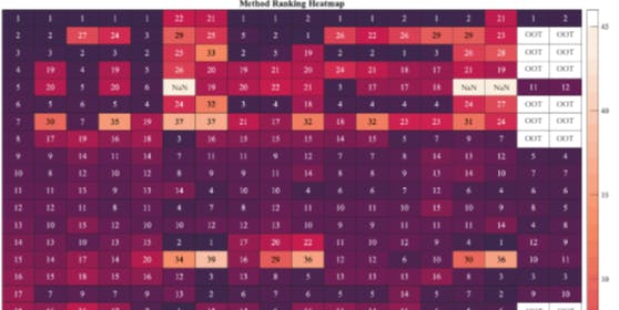
![Figure 7: Rankings of the linearization accuracy of 44 distinct methods for voltage magnitudes across various test conditions. The color intensity and labels used here have the same meanings as in Fig. 6. See Figs. 2, 3, 4, 5 and those in the supplementary file [55] for the specific ranking results, including mean and maximum relative errors for every method under each test case.](https://hackernoon.imgix.net/images/fWZa4tUiBGemnqQfBGgCPf9594N2-kke34uz.png?auto=format&fit=max&w=1920)
coordinate transformation are no longer linear representations of conventional variables but are linear representations of nonlinear mappings of these variables. Consequently, such models might be incompatible with the framework of decision-making problems such as unit commitment.
• Method PLS_CLS, unsophistically designed in this paper to simply illustrate the modular architecture of DPFL, demonstrates surprising accuracy with a superior ranking. Given its significantly lower complexity compared to the RR_KPC approach, the performance of PLS_CLS implies the considerable potential inherent in investigating the optimal ensemble strategy for the architectural configuration of DPFL.
• In the presence of individual data noise or outliers within the dataset, the reliability of clustering based and coordinate-transformation-based DPFL approaches is compromised. In these cases, alternative methods such as the method DLPF_C for voltage calculation, or the methods PLS_NIP, PLS_REC, DLFP_C, LS_COD, and LS_PIN for active branch flow calculation, are more reliable. It is important to note that although these methods are ranked between 4th and 15th, the differences in error among their resulting models are minimal. For instance, in the case of 33- bus-S-PF, the mean and maximal relative errors for the methods PLS_NIP, PLS_REC, DLFP_C, LS_COD, and LS_PIN are indistinguishable, as shown in Fig. 2.
• Regardless of the consistency in the rankings of certain methods, there is a notable degradation in the accuracy of all DPFL methods when exposed to individual data noise/outliers. E.g., as observed in Fig. 2 and 3, the mean and maximal errors for all DPFL approaches increase by one to three orders of magnitude in the case with data noise, as opposed to the noise-free condition. Such error amplification is uniformly observed across all test cases exposed to individual data noise/outliers. These results highlight the importance of the data cleaning process, e.g., filtering noise and outliers prior to data training.
• The results presented in Figs. 6 and 7 indicate that individual data noise/outliers yield a more significant influence on the performance of most approaches compared to joint data noise/outliers. This observation emphasizes the importance of transparency in research publications regarding the methodologies employed for introducing noise and outliers into datasets, not only to ensure clarity but also reproducibility. Henceforth, the term “noise/outliers” will be used to specifically denote individual data noise/outliers unless otherwise specified.
5.4.3. DPFL Performance: Individual View
The comparison of all methods reveals extensive information, particularly when focusing on some specific methods. Therefore, in the following, we present performance analyses of particular methods from their individual perspectives.
LS, LS_CLS, and LS_REC
First, the core of these three approaches is the original least squares method, which inherently has difficulties with multicollinearity, leading to frequent failures in our experiments. However, this does not imply a uniform failure across all scenarios, as in some instances, multicollinearity is less apparent. For example, in certain cases like 14-bus-S and 14-bus-L, the original dataset inherently does not have multicollinearity issues. Moreover, the introduction of data noise or outliers on an individual basis for every predictor can mitigate the interdependence among predictors, effectively addressing the multicollinearity issue. In such situations, as observed in 33-bus-S-NI, 33-bus-S-OI, 118-bus-L-NI, and 118-bus-L-OI, the methods LS, LS_CLS, and LS_REC did not fail, as indicated in Figs. 6 and 7.
Second, the LS_REC method begins its updates from a model initially derived through the LS approach using a subset of the training data, referred to as the old dataset. In contrast, the LS and LS_CLS methods utilize the entire training dataset, encompassing both the old and new datasets, for their training. This difference contributes to the inconsistent performance outcomes among these three methods. For instance, in the 14-bus-S test case, LS_REC encountered failure (as indicated in Figs. 6 and 7), due to multicollinearity within the old dataset. On the other hand, LS and LS_CLS did not fail as expanding the old dataset with new data eliminates the multicollinearity issue, illustrating that an increase in dataset size can potentially mitigate such issues. However, this phenomenon does not universally apply. For example, in the 118-bus-S case, the old dataset did not exhibit multicollinearity, allowing LS_REC to perform successfully. Conversely, incorporating new data into the dataset led to LS and LS_CLS failing due to the emergence of multicollinearity. This observation suggests that while altering the dataset size can influence multicollinearity, it offers no certainty regarding whether it will worsen or lessen the issue.
LS_TOL and LS_SVD


Likewise, method LS_SVD exhibited bad performance in test cases. This is primarily due to multicollinearity within the predictor’s training data, which can result in the Gram matrix having zero singular values. Consequently, a classical outcome of SVD — the 𝑺 matrix — may be extremely close to singularity. This near-singular condition significantly hinders the inversion accuracy of this matrix when implementing LS_SVD, leading to substantial errors.
LS_LIFX and LS_LIFXi
The LS_LIFXi method is the original version proposed in [15]. It specifically involves lifting each dimension of the predictor on an individual basis using different lift-dimension functions, as given in equations (11)-(15) of [15]. Note that LS_LIFXi draws inspiration from the dimension-lifting concept introduced in [16]. Yet, according to our understanding, the approach described in [16] jointly lifts all dimensions of the predictor using one lift-dimension function, rather than doing so individually with multiple lift-dimension functions. To respect the original concept in [16], we have also employed the LS_LIFX method in this paper. As seen from the evaluation in Figs. 6 and 7, LS_LIFX often demonstrates an improvement over LS_LIFXi, particularly in scenarios without data noise or outliers. This observation suggests that lifting all dimensions of the predictor jointly may yield enhanced results when the data is clean, though the error difference between the two methods is minimal.
LS_HBLD and LS_HBLE
In theory, methods LS_HBLD and LS_HBLE are expected to yield identical outcomes since both methods address a convex optimization problem and the transformations they adopt are equivalent. Practically, the results from LS_HBLD and LS_HBLE are also regarded as indistinguishable. Although their rankings might not be consistently next to each other, as illustrated in Figs. 2-5, the difference in their error magnitudes is minimal and can be attributed primarily to numerical inaccuracies, such as rounding errors.
Additionally, the two methods are specifically designed to address data outliers, including significant noise. They indeed have demonstrated improvements in accuracy when exposed to polluted data. For instance, in Fig. 7, in the test cases 33- bus-S-OI and 118-bus-L-OI, there is a notable enhancement in the rankings of both methods. Nevertheless, this trend is less apparent in Fig. 6. This difference may be attributed to the nature of the data involved: active branch flow data exhibit greater variability and sudden changes compared to voltage data. Consequently, applying a threshold to differentiate between normal data points and outliers, the core idea of LS_HBLD and LS_HBLE, will be more effective for voltage data (Fig. 7) than for active branch flow data (Fig. 6).
SVR, SVR_RR, and SVR_POL
First, as depicted in Figs. 6 and 7, the performance of methods SVR and SVR_RR is notably similar in most instances. This similarity primarily stems from the regularization factor for SVR_RR, which is configured to be as small as that in conventional methods like RR. A larger regularization factor can result in differences.
Additionally, SVR_POL offers no distinct advantages over SVR for two major reasons. Firstly, in situations where the underlying power flow data structure is nearly linear, the benefit of a polynomial kernel declines, leading to similar performance between SVR_POL and SVR with a linear kernel. Secondly, kernel selection is inherently challenging; while a 3rd-order polynomial kernel is a standard choice within the reproducing Hilbert kernel space, it may not effectively enable a highly linear representation of the projected power flow model.
Furthermore, methods SVR, SVR_RR, and SVR_POL should be robust to data outliers. This holds for the calculation of the voltage, as shown in Fig. 7, where these three methods show a large improvement in the rankings under the cases with data outliers, e.g., 33-bus-S-OI and 118-busL-OI. However, such an improvement is less obvious when computing active branch flows, as shown in Fig. 6. Similar to methods LS_HBLD and LS_HBLE, methods SVR, SVR_RR, and SVR_POL use a threshold to distinguish between data outliers and normal data points. Such a manner may be ineffective when large fluctuations exist in the dataset, such as the dataset of active branch flows.
Moreover, methods SVR, SVR_RR, and SVR_POL are designed to be robust against data outliers. Their effectiveness is evident in voltage calculations, as shown in Fig. 7: in test cases with data outliers, such as 33-bus-S-OI and 118-busL-OI, these three methods significantly outperform others. However, this enhancement is less pronounced in the computation of active branch flows, as illustrated in Fig. 6. Similar to LS_HBLD and LS_HBLE, SVR, SVR_RR, and SVR_POL employ a threshold to differentiate between outliers and typical data points. One threshold may be insufficient for datasets with extensive fluctuations, like those encountered in active branch flow data. In other words, effectively tuning this threshold can be challenging for such datasets.
PLS_BDL and PLS_BDLY2
First, as previously explained, the multicollinearity problem is more evident in PLS_BDLY2 than in PLS_BDL, due to the improper placement of the active power injection at the slack bus. This explains the failure of PLS_BDLY2 in specific situations where PLS_BDL remains effective.
Second, PLS_BDL and PLS_BDLY2 exhibit poor performance as indicated in both Figs. 6 and 7, which can be attributed to the presence of constant columns in the training dataset — as indicated in Table 4, generator terminal voltages are fixed, resulting in these constant columns. Due to their reliance on the bundle strategy, as outlined in [6], PLS_BDL and PLS_BDLY2 cannot handle these constant features effectively. This is because, again, the presence of constant columns disrupts the invertibility of a crucial matrix within their computational framework, thereby compromising the performance of these methods. However, introducing noise or outliers into the data — whether individual noise/outliers or joint noise/outliers — alters this condition, since the constant columns are disrupted by such data irregularities, which improves the invertibility of the aforementioned critical matrix. Consequently, in test cases such as 33-bus-S-NI, 33- bus-S-OI, 33-bus-L-NJ, 33-bus-L-OJ, 118-bus-L-NI, and 118-bus-L-OI, both PLS_BDL and PLS_BDLY2 exhibit enhanced performance compared to their results in other cases.
LCP_COU and LCP_COUN
In Fig. 6, the superior performance of LCP_COU over LCP_COUN can be attributed to the integration of real physical relationships into the LCP_COU. Specifically, LCP_COU incorporates the ground truth that the signs of the coefficients corresponding to the terminal angles of a line should be opposite. This physical insight aids in finding a more accurate solution, highlighting the value of embedding real physics into the training for DPFL approaches.
LCP_BOX and LCP_BOXN
Contrary to the above scenario, LCP_BOXN outperforms LCP_BOX according to Fig. 7. This difference in performance can likely be traced back to the nature of the physical knowledge incorporated into LCP_BOX. The information embedded in LCP_BOX is derived from a physics-based linear approximation, which does not equate to actual ground truth physical knowledge. Introducing this approximated physical knowledge does not necessarily enhance accuracy and, as observed in our study, can even be harmful. This suggests that the effectiveness of incorporating physical knowledge into DPFL training is highly dependent on the precision of that knowledge.
LCP_JGD and LCP_JGDN


This paper is available on arxiv under CC BY-NC-ND 4.0 Deed (Attribution-Noncommercial-Noderivs 4.0 International) license.


