EXPLORING THE CAPABILITY OF A
SELF-SUPERVISED CONDITIONAL IMAGE
GENERATOR FOR IMAGE-TO-IMAGE TRANSLATION
WITHOUT LABELED DATA: A CASE STUDY IN
MOBILE USER INTERFACE DESIGN
by
Hailee Kiesecker
A thesis
submitted in partial fulfillment
of the requirements for the degree of
Master of Science in Computer Science
Boise State University
March 2023
© 2023
Hailee Kiesecker
ALL RIGHTS RESERVED
BOISE STATE UNIVERSITY GRADUATE COLLEGE
of the thesis submitted by
Hailee Kiesecker
Thesis Title: Exploring the Capability of a Self-Supervised Conditional Image Gener ator for Image-to-Image Translation Without Labeled Data: A Case Study in Mobile User Interface Design
Date of Final Oral Examination: 10 March 2023
The following individuals read and discussed the thesis submitted by student Hailee Kiesecker, and they evaluated the presentation and response to questions during the final oral examination. They found that the student passed the final oral examination.
Timothy Andersen, Ph.D. Chair, Supervisory Committee
Casey Kennington, Ph.D. Member, Supervisory Committee
Edoardo Serra, Ph.D. Member, Supervisory Committee
The final reading approval of the thesis was granted by Timothy Andersen, Ph.D., Chair of the Supervisory Committee. The thesis was approved by the Graduate College.
ACKNOWLEDGMENTS
A long time coming but not a moment too soon.
I would like to share my gratitude for everyone in my life who helped guide me to where I am today. I would like to express my gratitude to Dr. Andersen for his patience and belief from the beginning that this was something I could accomplish. I would also like to acknowledge and appreciate my chaperons, who without them I don’t believe I could have found the courage to finish this research.
ABSTRACT
This research investigates the effectiveness of a conditional image generator trained on a restricted number of unlabeled images for image-to-image translation in computer vision. While previous research has focused on using labeled data for image labeling in conditional image generation, this study proposes an original framework that utilizes self-supervised classification on generated images. The pro posed approach, which combines Conditional GAN and Semantic Clustering, showed promising results. However, this study has several limitations, including a limited dataset and the need for significant computational power to generate a single UI design. Further research is needed to optimize the performance of the proposed approach for real-world applications.
TABLE OF CONTENTS
ABSTRACT………………………………………..
LIST OF TABLES……………………………………
LIST OF FIGURES…………………………………..
LIST OF ABBREVIATIONS ……………………………
1 INTRODUCTION …………………………………
1.1 Previous Work in Conditional GANs . . . . . . . . . . . . . . . . . . . . . . . . . . .
1.2 Previous Work in Image-to-Image Translation. . . . . . . . . . . . . . . . . . . .
1.2.1 Sketch Recognition and Completion . . . . . . . . . . . . . . . . . . . . . .
1.2.2 Sketch-to-Image Translation . . . . . . . . . . . . . . . . . . . . . . . . . . . .
1.2.3 Introducing Swire . . . . . . . . . . . . . . . . . . . . . . . . . . . . . . . . . . . .
2 METHODOLOGIES………………………………..
2.1 Dataset Selection:RICO . . . . . . . . . . . . . . . . . . . . . . . . . . . . . . . . . . . .
2.2 Architecture of the Conditional Generator. . . . . . . . . . . . . . . . . . . . . . .
2.3 Semantic Clustering using Nearest Neighbors. . . . . . . . . . . . . . . . . . . . .
2.4 Architecture of the Siamese Neural Network . . . . . . . . . . . . . . . . . . . . .
2.4.1 The Swire Sketch U I Dataset . . . . . . . . . . . . . . . . . . . . . . . . . . .
2.5 Show casing the Conditional GAN . . . . . . . . . . . . . . . . . . . . . . . . . . . . .
3 RESULTS ……………………………………….
3.1 Conditional Generative Adversarial Network Results. . . . . . . . . . . . . . .
3.2 Semantic Clustering Results. . . . . . . . . . . . . . . . . . . . . . . . . . . . . . . . . .
3.3 Showcasing the Conditional GAN Results . . . . . . . . . . . . . . . . . . . . . . .
4 DISCUSSION…………………………………….
REFERENCES………………………………………
A Model Parameters………………………………….
A.1 Pretext Model Training Parameters . . . . . . . . . . . . . . . . . . . . . . . . . . . .
A.2 Semantic Clustering Model Training Parameters . . . . . . . . . . . . . . . . . .
A.3 Self-Labeling Model Training Parameters. . . . . . . . . . . . . . . . . . . . . . . .
A.4 Generative Adversarial Training Network. . . . . . . . . . . . . . . . . . . . . . . .
B Reference Images for Results Chapter …………………..
LIST OF TABLES
1.1 Table of Ada IN reference variables. . . . . . . . . . . . . . . . . . . . . . . . . . . . .
2.1 Description of notation used in FID score equation.. . . . . . . . . . . . . . . .
2.2 Explanation of notation for SCAN loss equation.. . . . . . . . . . . . . . . . . .
2.3 Table describing the notation used in triplet loss. . . . . . . . . . . . . . . . . .
3.1 Classification Results . . . . . . . . . . . . . . . . . . . . . . . . . . . . . . . . . . . . . . .
LIST OF FIGURES
1.1 Parameter 00: A Car. Parameter 01: A Red Car. . . . . . . . . . . . . . .
1.2 Sample implementation of using the public Sketch-RNN software to
complete a sketch of a duck . . . . . . . . . . . . . . . . . . . . . . . . . . . . . . . . . .
1.3 Sample query and results Swire [12] . . . . . . . . . . . . . . . . . . . . . . . . . . . .
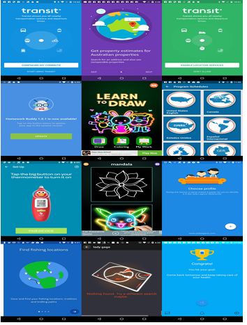
2.1 Set of RICO Screenshots. . . . . . . . . . . . . . . . . . . . . . . . . . . . . . . . . . . . .
2.2 Encoding of image class properties, enabling explicit control . . . . . . . . .
2.3 Basic flow of the pretext task for image classification. . . . . . . . . . . . . . .
2.4 The Siamese Neural Network has two twin ResNet50 CNNs whose weights are being updated individually based on embedding distance from sister network. The objective function is to minimize the distance between known positive images while maximizing the distance from known negatives. . . . . . . . . . . . . . . . . . . . . . . . . . . . . . . . . . . . . . . . . . .
2.5 Sample generation of anchor-positive pairs along with their negative pair, randomly sampled from the image class with the least similarity measured by Euclidean distance. Triplet loss is a loss function used in training neural networks for learning similarity between data points. It is often used in tasks such as face recognition and image retrieval. The idea is to enforce that features from similar images are closer in the feature space than features from dissimilar images. . . . . . . . . . . . . .
2.6 Example positive anchor pair. Left: Sketched UI layout from SWIRE dataset Right: Corresponding Real UI layout based on RICO ID. . . . .
2.7 Example positive anchor pair. Left: Sketched UI layout from SWIRE dataset Right: Corresponding Real UI layout based on RICO ID. . . . .
2.8 Novel Framework for Conditional GAN on a limited dataset without any image data labels. Where StyleGAN2 is our conditional image generator. SCAN is our clustering classifier. . . . . . . . . . . . . . . . . . . . . .
3.1 Full Process of Research Framework. Parameter Passing i.e. Sketch Image Input. . . . . . . . . . . . . . . . . . . . . . . . . . . . . . . . . . . . . . . . . . . . . . .
3.2 Generator generated images at generator initialization. FID Score 289 .
3.3 Generated Training GAN Loss and Entropy by Batch . . . . . . . . . . . . . .
3.4 Generator generated images at epoch 150. FID Score 57 . . . . . . . . . . . .
3.5 Transfer learning model image generations at FID 12.76.. . . . . . . . . . . .
3.6 Results of FID score over 04 days 02 hours and 58 seconds on 4 GPUs, peak FID score of 17.52. . . . . . . . . . . . . . . . . . . . . . . . . . . . . . . . . . . . . .
3.7 Transfer learning results of FID score over 04 days 02 hours and 56 seconds on 4 GPUs, peak FID score of 12.76.. . . . . . . . . . . . . . . . . . . . .
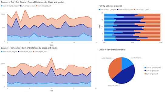
3.8 Average distance between clusters of datasets for model weights (ima genet, scan, selflabel), pie chart shows proportional distance between models for datasets . . . . . . . . . . . . . . . . . . . . . . . . . . . . . . . . . . . . . . . . .
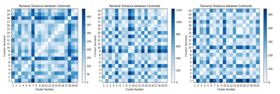
3.9 Visually depicts the average distance between each class for top 12 dataset . . . . . . . . . . . . . . . . . . . . . . . . . . . . . . . . . . . . . . . . . . . . . . . . . .
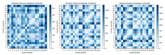
3.10 Visually depicts the average distance between each class for Generated Images dataset . . . . . . . . . . . . . . . . . . . . . . . . . . . . . . . . . . . . . . . . . . . .
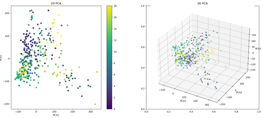
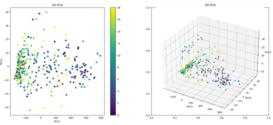
3.11 Top 12- Depiction of the location of the clusters within the space using ImageNet weights for ResNet50 . . . . . . . . . . . . . . . . . . . . . . . . . . . . . . .
3.12 Top 12- Depiction of the location of the clusters within the space using Semantic Clustering by Adopting Neariest Neighbors (SCAN) weights for ResNet50. . . . . . . . . . . . . . . . . . . . . . . . . . . . . . . . . . . . . . . . . . . . . .
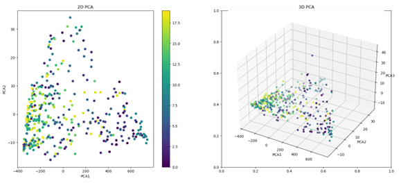
3.13 Top 12- Depiction of the location of the clusters within the space using Self Label weights for ResNet50 . . . . . . . . . . . . . . . . . . . . . . . . . . . . . . .
3.14 Generated- Depiction of the location of the clusters within the space using ImageNet weights for ResNet50 . . . . . . . . . . . . . . . . . . . . . . . . . .
3.15 Generated- Depiction of the location of the clusters within the space using (SCAN) weights for ResNet50 . . . . . . . . . . . . . . . . . . . . . . . . . . . .
3.16 Generated- Depiction of the location of the clusters within the space using Self Label weights for ResNet50 . . . . . . . . . . . . . . . . . . . . . . . . . .
3.17 Evaluation of Semantic Clustering Models 10 parallel Heads, Head 8 was found to be the best sampled starting point for RICO image clustering. . . . . . . . . . . . . . . . . . . . . . . . . . . . . . . . . . . . . . . . . . . . . . . . .
3.18 Evaluation of Self-Labeling task transferred off of Head 8 semantic model.
3.19 Distribution of Validation RICO set to Semantic Clusters. . . . . . . . . . .
3.20 left Distribution Classifications of enRICO dataset. right Distribution of Classifications of Generated Images . . . . . . . . . . . . . . . . . . . . . . . . . .
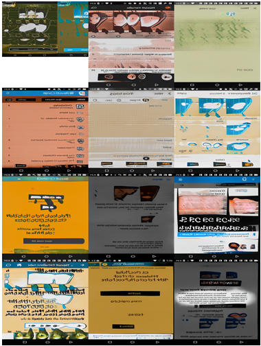
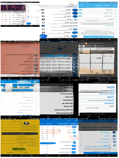
3.21 Sample of Generated Images in Cluster 15- Lines up with enRICO human labeled classification of ”list”. . . . . . . . . . . . . . . . . . . . . . . . . . . .
3.22 Confidence of the semantic clusters for each class . . . . . . . . . . . . . . . . .
3.23 Top 12 RICO Images in Cluster 0 . . . . . . . . . . . . . . . . . . . . . . . . . . . . .
3.24 Top 12 Generated Images in Cluster 0 . . . . . . . . . . . . . . . . . . . . . . . . . .
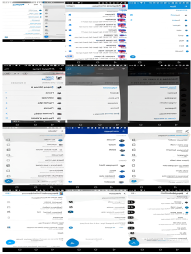
3.25 Top 12 RICO Images in Cluster 1 . . . . . . . . . . . . . . . . . . . . . . . . . . . . .
3.26 Top 12 Generated Images in Cluster 1. . . . . . . . . . . . . . . . . . . . . . . . . .
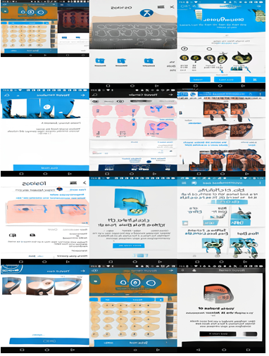
3.27 Top 12 RICO Images in Cluster 2 . . . . . . . . . . . . . . . . . . . . . . . . . . . . .
3.28 Top 12 Generated Images in Cluster 2. . . . . . . . . . . . . . . . . . . . . . . . . .
3.29 The classification process for a given Users ketch. . . . . . . . . . . . . . . . . .
3.30 Sample 00 User free hand sketch. . . . . . . . . . . . . . . . . . . . . . . . . . . . . . .
3.31 Sample 00 top 3 images of most confident cluster. . . . . . . . . . . . . . . . . .
3.32 Sample 00 top 3 images of second most confident cluster. . . . . . . . . . . .
3.33 Sample 00 top 3 images of least confident cluster. . . . . . . . . . . . . . . . . .
B.1 GAN trained to point of mode collapse, shows 120 generated images
that are nearly identical with each other.. . . . . . . . . . . . . . . . . . . . . . . .
B.2 Top 12 RICO Images in cluster 3. . . . . . . . . . . . . . . . . . . . . . . . . . . . . .
B.3 Top 12 RICO Images in cluster 4. . . . . . . . . . . . . . . . . . . . . . . . . . . . . .
B.4 Top 12 RICO Images in cluster 5. . . . . . . . . . . . . . . . . . . . . . . . . . . . . .
B.5 Top12 RICO Images in cluster 6. . . . . . . . . . . . . . . . . . . . . . . . . . . . . .
B.6 Top 12 RICO Images in cluster 7. . . . . . . . . . . . . . . . . . . . . . . . . . . . . .
B.7 Top 12 RICO Images in cluster 8. . . . . . . . . . . . . . . . . . . . . . . . . . . . . .
B.8 Top 12 RICO Images in cluster 9. . . . . . . . . . . . . . . . . . . . . . . . . . . . . .
B.9 Top 12 RICO Images in cluster 10. . . . . . . . . . . . . . . . . . . . . . . . . . . . .
B.10 Top 12 RICO Images in cluster 11. . . . . . . . . . . . . . . . . . . . . . . . . . . . .
B.11 Top 12 RICO Images in cluster 12. . . . . . . . . . . . . . . . . . . . . . . . . . . . .
B.12 Top 12 RICO Images in cluster 13. . . . . . . . . . . . . . . . . . . . . . . . . . . . .
B.13 Top 12 RICO Images in cluster 14. . . . . . . . . . . . . . . . . . . . . . . . . . . . .
B.14 Top 12 RICO Images in cluster 15. . . . . . . . . . . . . . . . . . . . . . . . . . . . .
B.15 Top 12 RICO Images in cluster 16 . . . . . . . . . . . . . . . . . . . . . . . . . . . . .
B.16 Top 12 RICO Images in cluster 17 . . . . . . . . . . . . . . . . . . . . . . . . . . . . .
B.17 Top 12 RICO Images in cluster 18 and 19 . . . . . . . . . . . . . . . . . . . . . . .
B.18 Randomly Sampled Generated U I Images in cluster 3 . . . . . . . . . . . . . .
B.19 Randomly Sampled Generated U I Images in cluster 4 . . . . . . . . . . . . . .
B.20 Randomly Sampled Generated U I Images in cluster 5 . . . . . . . . . . . . . .
B.21 Randomly Sampled Generated U I Images in cluster 6 . . . . . . . . . . . . . .
B.22 Randomly Sampled Generated U I Images in cluster 7 . . . . . . . . . . . . . .
B.23 Randomly Sampled Generated U I Images in cluster 8 . . . . . . . . . . . . . .
B.24 Randomly Sampled Generated U I Images in cluster 9 . . . . . . . . . . . . . .
B.25 Randomly Sampled Generated U I Images in cluster 10 . . . . . . . . . . . . .
B.26 Randomly Sampled Generated U I Images in cluster 11 . . . . . . . . . . . . .
B.27 Randomly Sampled Generated U I Images in cluster 12 . . . . . . . . . . . . .
B.28 Randomly Sampled Generated U I Images in cluster 13 . . . . . . . . . . . . .
B.29 Randomly Sampled Generated U I Images in cluster 14 . . . . . . . . . . . . .
B.30 Randomly Sampled Generated U I Images in cluster 15 . . . . . . . . . . . . .
B.31 Randomly Sampled Generated U I Images in cluster 16 . . . . . . . . . . . . .
B.32 Randomly Sampled Generated U I Images in cluster 17 . . . . . . . . . . . . .
B.33 Randomly Sampled Generated U I Images in cluster 18 and 19 . . . . . . .
LIST OF ABBREVIATIONS
UI–
User Interface
GAN–
Generative Adversarial Network
FID–
Frechet Inception Distance
RNN–
Recurrent Neural Network
SGD–
Stochastic Gradient Descent Optimizer
CHAPTER 1
INTRODUCTION
The purpose of this research is to investigate the capability of a conditional image generator trained on a restricted number of unlabeled images. While prior research has explored the challenge of image labeling for conditional image generation using substantial amounts of labeled data, this study focuses on the issue of training a conditional image generator without labeled images. Image-to-image translation is a computer vision task that maps an input image to an output image. The key contribution of this research is an original framework that can perform self-supervised classification on generated images, which can assist in image-to-image translation problems in computer vision.
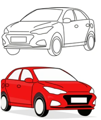
The use of Generative Adversarial Networks (GANs) has become popular in generating images, reducing image labeling costs, creating art, and natural language processing. Conditional GANs allow researchers to specify features of a generated image. For example, a conditional GAN can generate a red car image when given a parameter specifying the car and the color red. Figure 1.1 outlines this example. However, the lack of labeled images poses a significant challenge in current conditional GAN training methodologies.
To showcase the capability of a conditional GAN without labeled images, this research focuses on an image-to-image translation problem to aid in the freehand
wireframing process for mobile User Interface (UI) design. The aim is to generate realistic UI images that can be labeled in a self-supervised fashion using a user’s sketch of a mobile UI layout as a conditional parameter.
In mobile application design, there is a shortage of labeled mobile UI layout images. Additionally, collection and labeling of these images are a laborious task that requires researchers to take screenshots of various mobile applications and manually label each screenshot. Training a conditional GAN to generate UI layouts with current research methodologies would not be possible.
To overcome the limitations of conditional GANs’ requirement for labeled data, this research employs a combination of techniques, including StyleGAN2Ada- Py Torch, a leading GAN model with unsupervised separation of high-level attributes, and Semantic Clustering using Nearest Neighbors, an unsupervised clustering task with a limited feature vector capacity. Both techniques use image augmentation to identify their chosen features.
The research questions addressed in this thesis are:
• Can a GAN with limited training data generate realistic UI layout images, measured by the FID Score? (see Section 2.2)
• How accurately can we cluster GAN-generated UI layouts when trained on limited image data with no ground truth image classifications?
• How can a conditional GAN train on no labeled image data map a user’s input sketch to a generated UI layout?
The remaining sections of the study are presented in the following order. First, the fundamental background information is introduced, which encompasses previous studies on Generative Adversarial Network and semantic clustering. Next, the methods chapter breaks down the framework employed to examine the ability of a conditional image generator, trained on a limited amount of unlabeled data, to solve image-to-image translation problems. Finally, the results and discussion of this novel methodology are presented. All supplementary materials referred to in this article are available in Appendix A and B.
1.1 Previous Work in Conditional GANs
Conditional Generative Adversarial Networks (GANs) have been a popular topic of research in computer vision and machine learning for several years. Ian Goodfellow et al. in 2014 [5] introduced the original GAN architecture and has since been improved and extended in several ways. One of the extensions to GANs is the use of conditional information to guide the generation process. This is achieved by conditioning the generator and discriminator on additional inputs, such as class labels, attributes, or images.
Early works in conditional GANs include the Conditional GAN (CGAN) intro duced by Mirza and Osindero in 2014 [20], and the Auxiliary Classifier GAN (AC GAN)introduced by Odena et al. in 2016 [21]. Labeled data allows CGANs generator to train on the class labels or attributes of the training data. The discriminator, in turn, is trained to differentiate between the real and fake samples, as well as to predict the class labels or attributes of the input data.
These models showed that adding conditional information can improve the quality and diversity of generated images and can also control specific aspects of the generated images. The application of CGANs has led to the generation of high-quality images, such as photo realistic faces, with control of specific attributes like hair color, age, or facial expression.
StyleGAN
More recently, there has been a growing interest in using StyleGANs for conditional image generation. StyleGAN is a state-of-the-art GAN architecture introduced by Kerras et al. in 2019[13]. It is designed to generate high-resolution images with fine-grained control over style and structure. The key contribution of StyleGAN is the use of adaptive instance normalization (AdaIN), which allows the generator to control the style of the generated images based on a style code.
Conditional Style GAN (CS-GAN) is a natural extension of Style GAN to the conditional setting. CS- GAN uses an additional input to condition the generator and discriminator on class labels or attributes. The conditional information is incorporated into the AdaIN layers of the generator, which allows the model to generate images with specific styles or attributes.
Adaptive Instance Normalization- Ada IN
The normalizing methodology of AdaIN was introduced in the paper ”Arbitrary Style Transfer in Real-time with Adaptive Instance Normalization” by Huang and Belongie in 2017 [11]. AdaIN is a technique used in deep learning for tasks such as style transfer and image-to-image translation that involve manipulating the appearance of images.
LET:
x = Input Feature Map
y = Style Reference Image
µ= Mean of x
σ =Standard Deviation of x
ν =Mean of y
ρ = Standard Deviation of y
Z =Normalized Feature Map
Table 1.1: Table of AdaIN reference variables
To use AdaIN, we first compute the mean (µ) and standard deviation (σ) of the input feature map (x) that we want to normalize. We then normalize x by subtracting the mean (µ) and dividing by the standard deviation (µ), which results in a normalized feature map (Z) that has a standard normal distribution, view Equation 1.1:
Z = x−µ by σ (1.1)
We can then calculate style information from a style reference image (y) to the normalized feature map (Z). Specifically, we use the mean (ν) and standard deviation (ρ) of y to scale and shift the normalized feature map, respectively, using affine transformations. This aligns the statistics of the style and content, allowing us to
transfer the style of the style image (y) to the content of the input image (x) yielding a Transformed Feature Map (W):
W =(ρ∗Z+ν) (1.2)
Here, W is the final feature map that has been transformed to match the style information. The parameters ρ and ν are learned during training and are specific to each channel of the feature map.
In summary, AdaIN is a technique for manipulating the appearance of images that involves normalizing the input feature map and adjusting it with style information using affine transformations.
StyleGAN2
In recent years, StyleGAN2 has become one of the most widely used models for conditional image generation. StyleGAN2, which was introduced by Kerras et al. IN 2020 [14] is an improved version of the original StyleGAN. It is designed to generate high-resolution images with even finer control over style and structure compared to
the original StyleGAN.
The conditional extension of StyleGAN2, known as Conditional StyleGAN2 (CS GAN2), has been used in various applications, such as domain adaptation [19], super resolution [7], and face synthesis [18]. In domain adaptation, CS-GAN2 is used to generate images in a target domain , given images in a source domain. In super resolution, CS-GAN2 is used to generate high-resolution images from low-resolution inputs. In face synthesis, CS-GAN2 is used to generate faces with specific attributes, such as age, gender, and emotion.
Recent research on CS-GAN2 has focused on improving the quality and diversity of generated images, and on making the model more robust and scalable [1], [30], [28], [24]. For example, researchers have proposed methods to incorporate additional information, such as semantic maps or reference images, into the generator. They
have also explored ways to improve the training stability and robustness of the model, and to extend it to more challenging tasks, such as video synthesis and interactive generation [25, 10, 24] . However, the requirement of supervised pre-training and labeled data has been a limiting factor for the use of CGANs, including CS-GAN2 [28, 30, 1].
Despite CGANs success, the requirement for labeled data has been a limiting factor for the widespread application of CGANs, including CS-GAN2. Recent studies have attempted to address the conditional limitation by exploring methods to train CGANs on unlabeled data [14].
Overall, the current research on CGAN and CS-GAN2 demonstrates conditional GANs potential for various applications in computer vision and machine learning and highlights the need for further improvement and exploration in this field.
1.2 Previous Work in Image-to-Image Translation
This study employs an image-to-image translation problem to assist in the freehand wire framing process for mobile user interface (UI) design. The main goal is to examine how well a type of machine learning model called a conditional GAN can learn to generate mobile user interface (UI) layouts from rough sketches drawn by a user, without using any pre-labeled or pre-classified training data. A basic comprehension of current image-to-image frameworks is pivotal for this task.
Hence, in this section, we will cover the Quick, Draw! dataset in 2017 [6] and the Sketch-RNN framework
in 2018 [22], which are important tools for training models for sketch recognition and completion. Additionally, we will discuss two other applications of sketch-to image translation: Interactive Sketch and Fill in 2019 [4] and StackGAN [29] in 2017. Finally, the section will present Swire [12], a deep learning-based sketch-to-existing UI layout retrieval system that assists designers in retrieving similar UIs from a dataset by providing a sketch of the desired UI layout.
1.2.1 Sketch Recognition and Completion
”Quick, Draw!” is a dataset created by Google researchers in 2016 that consists of millions of human-made freehand sketches in various categories, such as animals, objects, and everyday things. The aim of this project was to help train machine learning models for sketch recognition and classification tasks. This dataset serves as a crucial resource for training deep learning models to recognize and classify hand-drawn sketches. Sketch-RNN is a framework that was also developed by the same research team lead by David Ha to improve the process of completing users’ sketches.
Sketch-RNN 2017 is a novel deep learning framework that can complete a user’s partially drawn sketch by using a recurrent neural network (RNN). This framework is unique in that it generates a sketch sequentially, one stroke at a time, rather than in a single pass. The RNN is trained on the Quick, Draw! dataset to learn the
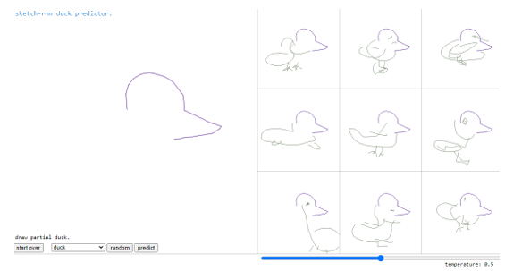
relationships between different strokes and generate new sketches that are consistent with the user’s drawing style.
The RNN used in Sketch-RNN is a two-layer, multi-directional Long Short-Term Memory (LSTM) network that is trained on the Quick, Draw! dataset. The model takes as input a sequence of strokes and outputs a new stroke for each time step. The output stroke is determined by a probability distribution that is learned during the training process. This distribution is based on the previous stroke, the hidden state of the RNN, and the parameters of the LSTM cell. The output is fed back into the RNN, which generates a new hidden state and new output. This process continues until the network outputs an ”end of sketch” token.
In addition to Sketch-RNN, Sketchforme [8] in 2019 is one of several neural network-based systems that can generate sketches based on user input. It uses a combination of Transformer, LSTM, heat-maps, and Gaussian Mixture Models (GMMs) to produce sketches of the given scenes. Another system, Scones [9] in 2020, has a similar architecture but employs a chat bot to develop multi-category sketch scenes.
Overall, the ”Quick, Draw!” dataset and Sketch-RNN framework represent a significant advance in the field of sketch recognition and completion. The combination of these two tools has opened new possibilities for machine learning applications that involve hand-drawn sketches. By training models on large datasets of human-made sketches, researchers can develop algorithms that are better at recognizing and gen erating drawings that are consistent with users’ styles. The potential applications of this technology are vast, including in fields such as art, design, and education.
1.2.2 Sketch-to-Image Translation
Sketch-to-image translation refers to a process where a neural network generates a realistic image based on a user’s sketched input. Interactive Sketch and Fill, proposed by Ghosh et al. in 2019 [4], is a two-stage Generative Adversarial Network (GAN) process that accomplishes sketch-to-image translation. In the first stage of this process, the user’s initial input stroke is used to generate an outline of the intended object, while in the second stage, a realistic image is produced based on the outline generated in the first stage.
Similarly, StackGAN [29] is a text-to-photo realistic image synthesis application that generates images from textual descriptions. This application uses two GANs to generate high-resolution images that are semantically meaningful based on a textual description of the object. In the first stage, low-resolution images are synthesized from the text description, while in the second stage, the generated images are refined to a higher resolution. The images produced by StackGAN are of high quality and have a realistic appearance.
Sketch-to-image translation is a challenging problem in machine learning, primarily because sketches often lack details and are often incomplete, leading to ambiguity in the intended object. Therefore, the success of such an application relies heavily on the ability of the neural network to recognize and complete the object based on the user’s input. The use of GANs is an effective method for overcoming the problem of sketch ambiguity, as they can generate realistic images by modeling their distributions.
In conclusion, Sketch-to-image translation is a challenging task but approaches such as Interactive Sketch and Fill and StackGAN are effective at generating high quality images that are semantically meaningful and resemble the user’s intended object. GANs are a promising method for tackling the problem of sketch ambiguity and generating realistic images.
1.2.3 Introducing Swire
Swire [12] in 2020 is a novel deep learning-based sketch-to-Image UI layout retrieval system. Its primary objective is to assist designers in retrieving similar UIs from a dataset by providing a sketch of the desired UI layout. Swire achieves this by utilizing a dataset of freehand UI layout sketches, which are used to train the system against RICO to learn the best matching UIs.
To achieve this goal, Swire employs two convolutional sub-networks with different weights, which handle the input of a sketch and UI pair. These sub-networks encode matching pairs of sketches and screenshots with similar values, allowing Swire to learn to recognize similar UI layouts from sketch input.
![Figure 1.3: Sample query and results Swire [12]](https://worldofsoftware.org/wp-content/uploads/2024/02/figure-1.3.png)
The dataset used by Swire is an essential component of the system, as it provides the necessary input to train the deep learning model. The Swire dataset includes approximately 3.3k sketches and utilizes the RICO dataset which was used to train the system. Learn more about RICO in Section 2.1 and Swire in Section 2.4.1. However, it is worth noting that a more extensive and diverse dataset could potentially improve the system’s accuracy.
In conclusion, Swire is an innovative system that utilizes deep learning techniques to provide designers with a tool for retrieving similar UIs from a dataset based on sketch input. The system’s ability to learn from a dataset and provide accurate results is a significant development in the field of UI design.
CHAPTER 2
METHODOLOGIES
This chapter will describe the methodology used in this research, including the selection of the dataset, the architecture of the conditional generator, the training procedure, and the evaluation metrics used.
2.1 Dataset Selection: RICO
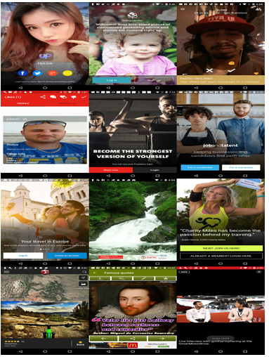
The Mobile UI RICO dataset [3] created in 2017 is a large dataset of user interface screens collected from Android mobile applications. It was created by researchers at the University of California, Berkeley to support research in UI design and development. The dataset contains more than 66,000 UI screens from over 9,000 unique mobile apps, see Figure 2.1 for an example. Each screen in the dataset is represented as a PNG image and is accompanied by metadata that includes the app name, screen title, screen category, and other relevant information.
The RICO dataset is unique in that it includes not only screens from popular and well-known apps but also less popular and niche apps. This makes it a valuable resource for researchers interested in studying UI design across a broad range of apps and use cases. In addition to the UI screens themselves, the RICO dataset also includes annotations of the UI elements on each screen, such as buttons, text fields,
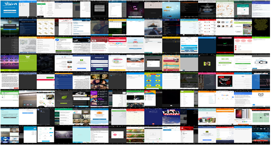
and images. These annotations were created by crowd-sourcing the task to workers on Amazon Mechanical Turk and were subsequently validated by experts in UI design. Overall, the Mobile UI RICO dataset is a valuable resource for researchers inter ested in mobile UI design, development, and evaluation. It has been used in a wide range of studies and research projects, including the development of machine learning algorithms for UI design and the analysis of design patterns in mobile apps [3, 16, 26].
For these reasons RICO was selected as the main dataset used in this research and was used to train the conditional GAN in this case study.
RICO Normalization
Upon experimentation, it was discovered that the images in the RICO dataset had varying sizes and color scales. These images were prepared with a resolution of 512×512 pixels on three color channels [3, 512, 512] to ensure a consistent format for future training.
2.2 Architecture of the Conditional Generator
Generative Adversarial Networks (GANs) are a type of neural network consisting of two competing convolutional networks, the generator, and the discriminator. The objective function of GANs involves maximizing the probability of correct data classification by the discriminator and minimizing the probability of incorrect data classification by the generator. See objective function in Equation 2.1.
MINGMAXD =Ex∼pdata(x)[log D(x)]+Ez∼pz(Z)[log(1 − D(G(z))] (2.1)
The limited availability of image data for training GANs has been a concern. However, StyleGAN2, a conditional GAN, can generate high-quality images on limited datasets while maintaining image realism. One of the significant breakthroughs of StyleGAN2 is the ability to learn a distribution of high-level attributes to ensure an even distribution of image generation variations and prevent mode collapse. The StyleGAN2 model can separate high-level attributes unsupervised, allowing for high quality image generation on a limited dataset. The Fr´echet Inception Distance score (FID) is a metric that measures the distance between feature vectors for real and generated images, and StyleGAN2 can train to a low FID score with a small image dataset.
Moreover, StyleGAN2 can learn image features and becomes conditional with parameter inputs when given a clean labeled dataset of images and their corresponding classifications. The equation for FID can be seen in Equation 2.3 its variables are described in Table 2.1.

(2.2)
d2((m,C),(mw,Cw)) = ||m −mw||2 2 + Tr(C +Cw −2(CCw)1/2), (2.3)
Notation Description
m Mean of feature activation’s for real images
mw Mean of feature activation’s for generated images
C Covariance matrix of feature activation’s for real images
Cw Covariance matrix of feature activation’s for generated images
Tr Trace of a matrix (sum of its diagonal elements)
|| · ||2 L2 (Euclidean) norm of a vector
Table 2.1: Description of notation used in FID score equation.

(2.4)
StyleGAN2’s division of the GANs latent space allows each subspace to encode an image class property, enabling explicit control over each property. The StyleGAN2 architecture divides two latent spaces, Z and W, into N+1 sub-spaces, with N being the number of attributes, and an additional attribute to compensate for immeasurable control properties. This can be seen in Figure 2.2. Having two latent spaces that correspond to each other leads to a cleaner representation of distinct class properties.
The loss function for StyleGAN2 is a contrastive loss that aims to ensure that similar images exist in latent space closer together. This is described in Equation 2.2. The loss function has a component for each attribute, defined in Equation 2.4. Where lkis a contrastive loss component for each attribute k.
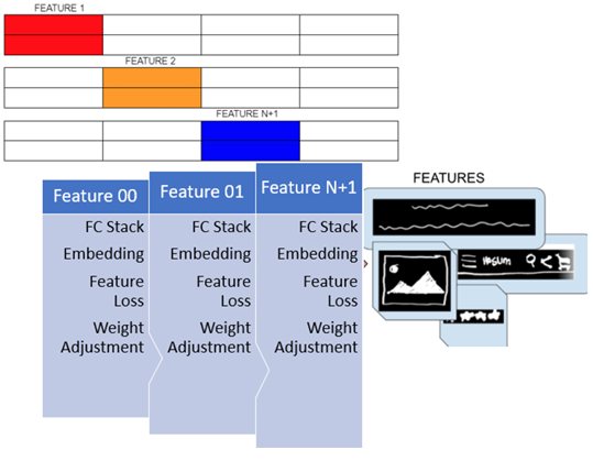
The mapping of generated images into Mk : I −→ RDk assumes that images with similar attributes will be found in Dk dimensional space close together. Clustering is a powerful method that leverages this assumption to group similar images into classes. Using clustering can improve the performance of GANs, especially when trained on a limited dataset.
In this research we took the RICO dataset and implemented semantic clustering on the image data. This methodology is explained in the following section.
2.3 Semantic Clustering using Nearest Neighbors
When training a conditional GAN, semantic clustering can help to improve the quality of the generated images by encouraging the generator to produce samples that are representative of each class of the conditional labels. This is particularly useful when working with a small image dataset because it can help to mitigate the problem of over-fitting and improve the diversity of the generated images.
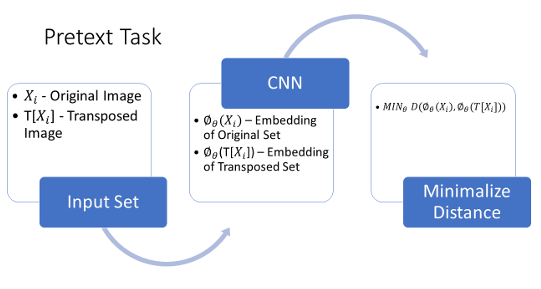
Semantic clustering is a process of unsupervised learning that uses image augmentations to group images into clusters based on their mapped latent space. This is achieved through a feature vector representation of the image, which represents high-level image features. The feature vector is created by performing a pretext task on the image, which is a form of representation learning. Pretext tasks use the invariance criterion to learn and generate qualitative feature representations.
MINθ D(ϕθXi,ϕθ(T[Xi])) (2.5)
Pretext tasks create a set of feature vectors by augmenting the original dataset, which minimizes the distance between original images Xi and their augmentations T[Xi]. The pretext task learns an image embedding in a self-supervised fashion ϕθ, allowing semantically similar images based on found meaningful characteristics to exist closer together in an embedding space. Equation 2.5 finds the minimum distance between original image X and its transposed copies, see Figure 2.3. The weights are then transferred from the pretext task using transfer learning, which establishes a better starting point in understanding the representation of important features for training. The next step is to use the trained instance discrimination model (Pretext Model- ϕθ) to mine all K nearest neighbors of images (Xi) in a set (D), from the embedding space. The neighboring image set is defined as images existing within the same cluster, which are likely part of the same semantic cluster but with varying accuracy in their classification.

(2.6)
To solve the issue of varying classification accuracy, the implemented semantic clustering model in this research used SCAN loss, see Equation 2.6 and Table 2.2. The model improves on clustering classifications by randomly augmenting the original image dataset and their found mined neighbors (Mining Model). The model uses the Stochastic Gradient Descent Optimizer (SGD) with momentum 0.9 and initial learning rate 5.0 with ten heads clustering into twenty different classifications. View Appendix A for full model arguments. SGD Optimizer is a popular optimization algorithm used in machine learning to update the parameters of a model in order to minimize the loss function. Since accuracy of the model greatly depends on starting point initiation, each of the ten heads represents a parallel training model with different starting parameters.
Choosing the head with the lowest loss is ideal because it led to a better performance in the semantic clustering process. The basic idea behind the SGD optimizer is to update the model parameters iteratively using the gradient of the loss function with respect to the parameters, computed on a subset of the training data, also known as a mini-batch.
After the Mining Model completes training, transfer learning is utilized to improve classification accuracy. The final model of the semantic clustering process collects the top-20 image classifications of each cluster and preforms the Mining task on each image (Self-Label Model). This final step greatly improves the classification accuracy of each cluster.

During the training of this research on the cleaned RICO dataset, the images were cropped to 256×256 pixels on three color channels [3, 256, 256]. A total of 1,342 images were set aside for testing, while 45,000 images were used for training. For all training steps, T[Xi], cropping transformations were performed, and normalization by mean and standard deviation was implemented.
In the pretext task, each batch consisted of 128 images, with 300 epochs and 20 potential clusters. The mining task utilized transfer learning from the pretext task, and was trained on a batch size of 128 with 100 epochs, maintaining 20 potential clusters. During the self-labeling task, the batch size remained at 128 images, with the number of potential classifications unchanged, and the number of epochs reduced to 75.
Semantic Clustering by adopting Nearest Neighbors [27], states the number of mined neighbors has minimal effect on the accuracy of the clusters. Therefore, the number of mined neighbors remained constant at 50 for each task. Furthermore, since the pretext task is aimed at solving an instance discrimination problem, the ResNet-50 model was selected as the backbone network.
The choice of the ResNet-50 model as the backbone network for the pretext task was selected because ResNet models have been shown to be highly effective at image recognition tasks, including instance discrimination. The ResNet-50 architecture has been specifically designed to enable deeper networks with improved performance, by addressing the problem of vanishing gradients that can occur in very deep networks. Therefore, given that the pretext task is focused on instance discrimination, selecting ResNet-50 as the backbone network is a logical choice that should help to ensure the best possible performance.
Once the images had been clustered, the conditional labels were assigned based on the cluster to which each image belongs. The resulting labels then can be used for the conditional GAN, with the goal of generating images that are representative of each semantic cluster.
By incorporating semantic clustering into the training process, the conditional GAN can learn to generate images that are not only visually appealing but also semantically meaningful. This can lead to better results, particularly when working with a small image dataset where overfitting is a concern. In this research the self labeling task implements Equation 2.5 on the top-20 most confident images in each of the clusters. Over fitting is avoided by using strong image augmentations of confident classifications examples.
In summary, this research implements StyleGAN2 to allow for high-quality image generation on a limited dataset, which is achieved by dividing the GANs latent space to enable explicit control over each property, and measured through FID score. Semantic clustering using nearest neighbors was implemented as it can improve the performance of GANs, particularly on a limited dataset, by grouping similar images into classes.
2.4 Architecture of the Siamese Neural Network
In the case study demonstrating the ability of a conditional GAN trained without labeled data to associate a sketched image with a realistic representation, a Siamese Neural Network was employed to learn the distance metric between these two image styles. This section explains the ability of a sketched image to be associated with a realistic representation, without any known ground truth labels for both the sketch and the generated image.
The Siamese Neural Network is a structure that includes two sister convolutional neural networks with a conjoined image encoding layer and distance measure, view Figure 2.4. Siamese networks have been used historically for object tracking and single-shot image recognition [2, 15]. For the classification task, the Siamese network employs an anchor-positive image
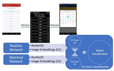
pair and an anchor-negative image pair. The goal is to measure the anchor-positive images closer together and the anchor-negative images further apart. This is achieved by generating a set of anchor-positive pairs and anchor negative pairs were randomly sampled from the image class with the least similarity, as shown in Figure 2.5. Sketches related to realistic images were trained with the distance between them minimized using triplet loss, which is a loss function that minimizes the distance between an anchor image and a positive image while maximizing the distance between an anchor image and a negative image. The triplet loss is computed over a set of triplets (xa
i, xp i, xn i), where xa i is an anchor image, xp i is a positive image (i.e., an image that is similar to the Anchor), and xn i is a negative image (i.e., an image that is dissimilar to the Anchor).
To evaluate the distance between each sketch image pair, the researchers compared
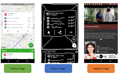
pair, randomly sampled from the image class with the least similarity measured by Euclidean distance. Triplet loss is a loss function used in training neural networks for learning similarity between data points. It is often used in tasks such as face recognition and image retrieval. The idea is to enforce that features from similar images are closer in the feature space than features from dissimilar images.
the distance between a positive anchor pair and the top 12 most confident samples from each of the 20 semantic clusters. This process involved using and evaluating four distance metrics: Euclidean, Cosine, Infinity, Manhattan, and Hamming.
||xa i − xp i||2 2 + α < ||xa i − xn i ||2 2,∀(xa i,xp i, xn i) ∈ T (2.7)
Triplet loss was chosen for the Siamese network during training due to its ability to outperform current in-place loss functions for image similarity problems. In a seminal work, researchers demonstrated that the use of triplet loss reduced the error between DeepFace, DeepID2, and Bag-of-Words Histogram of Oriented Gradients by

dataset Right: Corresponding Real UI layout based on RICO ID
x7, 30% [23], and 22.1% [12], respectively. It is important to note, however, that the reduction in error achieved with triplet loss depends on the specific network architecture being used [23]. Nevertheless, the use of triplet loss has become a standard practice for training Siamese networks, especially those aimed at solving image similarity problems, due to its effectiveness in this regard. Semi-hard negative images and semi-hard positive images are chosen from each input batch to help with learning progression. These images are chosen within a given
Notation Description
f(x) Function
d(x,y) Distance Metric (usually Euclidean distance)
α Margin
T Triplet set (set of all possible image triplets in the dataset)
Table 2.3: Table describing the notation used in triplet loss.
margin of error to minimize the likelihood of mode collapse. Mode collapse occurs when distances between image pairs begin to converge to zero, regardless of positive or negative status. Using an instance of a negative image that is greater than the distance of the found hard positive mitigates mode collapse from happening. The formula for the triplet loss function is shown in Equation 2.7 and outlined in Table 2.3.
The Siamese network structure uses two CNNs, one for an input sketch and one for a its reference image, to find a 64-dimensional vector output for both image instances, which are mapped in latent space together. Using Triplet loss maximizes the distance between the positive and negative anchor pairs. The average anchor-positive distance per batch of sketch-image pairs can be estimated, and this can be used to create a baseline distance of acceptability between images (dataset RICO) and sketches (dataset Swire see following subsection 2.4.1) that are already known. View Figure 2.7. Using the trained CNNs and Triplet loss function, the Siamese network can learn the distance metric between sketches and generated images without ground truth labels.
2.4.1 The Swire Sketch UI Dataset
Introduced in Previous Works Swire is a research paper that presents a dataset called the Sketch UI dataset Swire, which contains sketches of UIs from the RICO dataset.
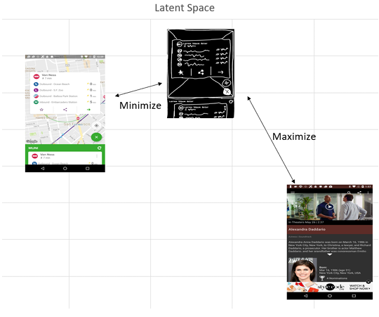
The paper describes the creation and characteristics of the Swire dataset, which has a one-to-one correspondence with the UIs from the RICO dataset via the image UI ID. The Swire dataset comprises 3,333 sketches of user interfaces that were created by four different sketchers, identified by anonymized sketcher IDs ranging from 1 to 4.
These sketches are provided as image files that have been inverted to grayscale, with values towards white representing artist strokes and values towards black representing the background. The paper emphasizes that Swire offers a valuable resource for researchers interested in developing and testing machine learning models for UI design
and analysis. An example can be seen in Figure 2.6 This research used the Swire dataset to train the Siamese model to learn the baseline distance between sketches and their realistic counterparts to help with conditional parameter passing.
2.5 Showcasing the Conditional GAN
This study aimed to demonstrate the effectiveness of a conditional GAN for image to-image translation tasks in the context of mobile user interface design, without the need for labeled images. Specifically, the study sought to generate realistic UI images that could be labeled in a self-supervised manner using a user’s wireframe sketch of
a mobile UI layout as a conditional parameter.
The research methodology involved training a Generative Adversarial Network, semantic clustering model, and Siamese neural network to enable a user to input a freehand wireframe layout sketch and identify the appropriate image classification. The distance was calculated based on the sketch against the top 12 identified image classifications from each of the 20 clusters, with the top 3 out of 20 classifications returned.
For each of the three image classifications, the image bank of GAN images returned 3 images in each classification within an appropriate margin of error. The margin of error ensured that the generated images were not too far away from or too close to the user’s sketch. The top-9 generated GAN images were returned to the user based on Euclidean distance calculated from the feature vector representations.
The generated images were effectively filtered with given sketch UIs, i.e., a Con ditional GAN without any image data labels. In the following chapter, the individual
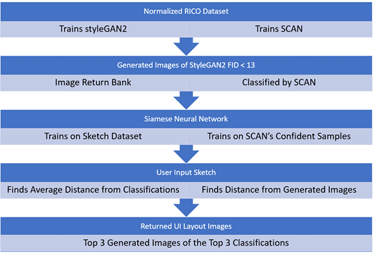
image data labels. Where StyleGAN2 is our conditional image generator. SCAN is
our clustering classifier.
results of trained GAN and clustering classifier will be presented. They are then evaluated on how well they were able to map a freehand sketch to a realistic image using no true labeled image data. Figure 2.8 provides a visualization of the entire process.
CHAPTER 3
RESULTS
This section presents the findings of our research, specifically regarding the quality of the generated images and the performance of the generator in terms of image translation.
Our methodology, view Figure 3.1, involves the use of a Generative Adversarial Network (GAN) that is trained on a set of real user interface (UI) images. Additionally, we trained a Semantic Clustering model on the same set of RICO images to group similar together.
Subsequently, the trained GAN was employed to generate new UI images, and the semantic clustering model was utilized to evaluate the quality of the generated images.
To further refine the generative process, we employed a conditional GAN architecture, which allowed for the generation of images based on certain characteristics while having no prior knowledge about the dataset. This was achieved using a Siamese network that utilized the weights of the trained clustering model to minimize the distance between sketch image pairs, resulting in conditional GAN images.
Overall, this approach presents a novel and effective solution to generating high quality UI images, despite the complexity and variability of the UI domain.
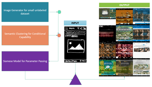
Input.
3.1 Conditional Generative Adversarial Network Results
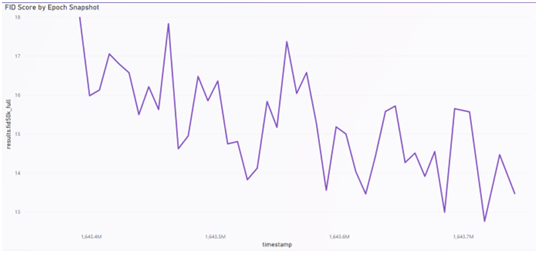
The Generative Adversarial Network (GAN) outlined in Section 2.2 was trained on the RICO dataset across 4 GPUs for a total of 4 days, 2 hours, and 58 seconds, and achieved a peak FID score of 17.52. The FID score is a metric that measures the similarity between the distribution of real images and generated images. Lower scores indicate better image quality.
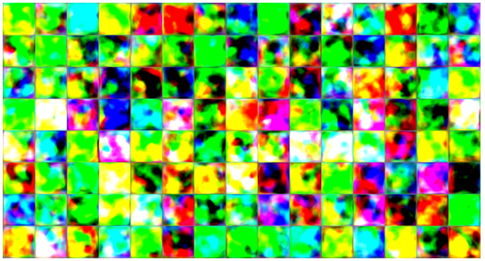
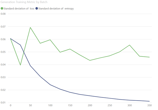
Figure 3.3, displays the models loss and entropy throughout the GANs training process on the RICO dataset. The figures below display generated images at various epochs during training, starting with initialization and training to FID 12.76 view Figure 3.2.
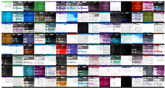
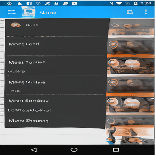
To improve the FID score with the goal being as close to 0 as possible. Meaning there is no dissimilarity between generated images and real images. Transfer learning was performed on the GAN,resulting in a drop of 4.76 points to a 12.76 FID score after 2,123 additional intervals. A good range for state of the art FID score for Generative Models is between 20- 10. The transfer learning model’s generated samples can be seen in Figure 3.5. The provided image samples show that the GAN was capable of finding major distinctions within a very specific image type.
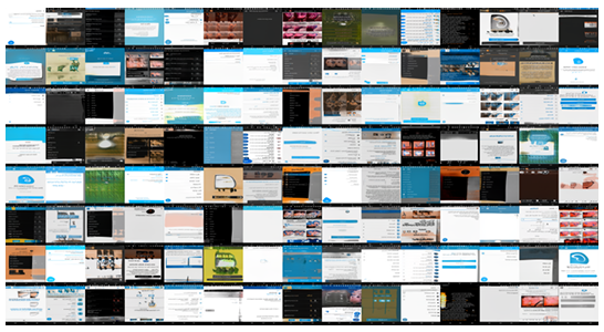
Evaluation of the graphs in Figures 3.6 and 3.7 demonstrates the steady improve ment of the convolutional network, even on a specialized small image dataset. The GAN is capable of generating a variety of User Interface layouts that are detailed enough for the wireframing design process, as shown in Figure 3.1 which displays generated wireframe designs with random seed inputs.
3.2 Semantic Clustering Results
The accuracy with which we can cluster GAN-generated UI layouts, when trained on limited image data with no ground truth image classifications, is contingent on the effectiveness of training our Semantic Clustering Model and assessing its ability to improve the classifications. Semantic Clustering also enables us to evaluate the performance of our Generative Adversarial Network in generating a diverse dataset with high-quality images.
In the pretext task, as outlined in Section 2.3, demonstrated a 100% accuracy for the top-50 nearest neighbors on the training set, which can be explained by the lack of ground truth annotations in the training images. However, the model’s accuracy score on the validation set of UI screenshots, which was obtained from the enRICO dataset, was only 32.91%. This dataset comprises 1,460 high-quality RICO UIs that have been manually classified into 20 distinct design topics, as described in [17].
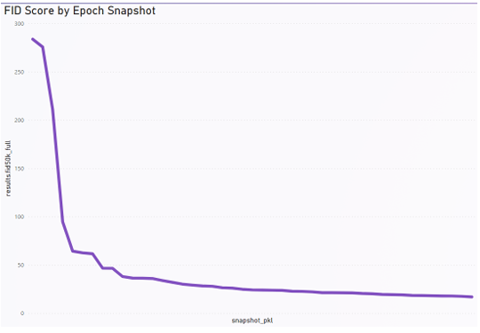
peak FID score of 17.52.
The validation set was used to evaluate the model’s performance during the training process. It should be noted, however, that the enRICO labeled dataset is not essential for the semantic clustering process and is used solely for the purpose of providing an accuracy evaluation.
To evaluate the quality of our image clustering model, the pairwise distance between each of the images in the individual clusters was calculated. This assessment was carried out on two datasets: first, the top 12 most confident samples of images from each of the 20 clusters, and second, generated images obtained from our trained Generative Adversarial Network. Figure 3.8 illustrates the average distance between each of the clusters. The labeled enRICO dataset is not necessary for this evaluation.
It is worth noting that a model’s ability to distinguish the similarity between image clusters improves as the average distance of its clusters increases. As can be seen in Figure 3.8, the loaded general model of RESNET50(weights = ’imagenet’) has an average cluster distance that is three times shorter than our self-labeling model.
This concept can be illustrated through the following heatmaps, Figure 3.9, in which the image set remains constant but the model responsible for generating feature vectors is altered. These heatmaps visually depict the average distance between each class, demonstrating that as the clustering process continued, the average distance between clusters for our top 12 images increased.
By examining the subsequent set of heatmaps, 3.16, for the generated images dataset, we can observe a significant similarity to the top 12 dataset. This indicates that our image generator is producing images that are sufficiently similar and distributed.
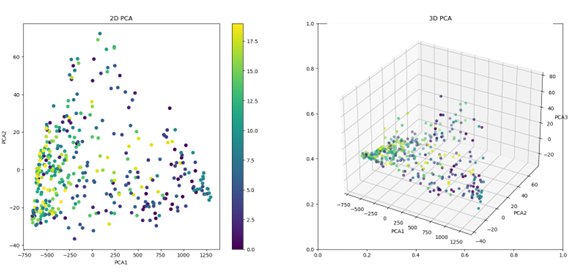
Our data can be represented visually in a 3-dimensional space, providing a more
accurate depiction of the location of the clusters within the space. It is noteworthy that for the top-12 dataset, we observe a high degree of similarity between the data clusters, which gradually shifts as the training process continues.
The same analysis can be performed for the generated images dataset, and the resulting images provide a similar visualization of the data clusters in 3-dimensional
space.
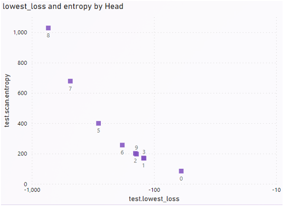
During the semantic clustering stage of the three-process clustering model, 10 linear heads were initialized in parallel. The head with the lowest loss was selected to proceed to the Self-Labeling process. Among the 10 heads, Head 8 had the lowest total
Images dataset
ImageNet weights for ResNet50
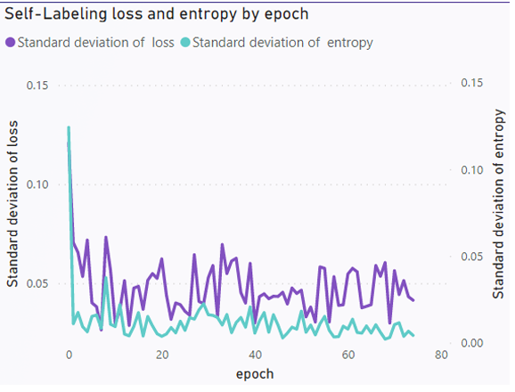
loss during the SCAN-loss cluster training, as shown in Figure 3.17. Head 7, which had a close follow-up based on the entropy value, was found to be the second-best choice, while Head 0 was the least adaptable to the image dataset. For the Self-Labeling task, we chose Head 8 to train against. We found that loss and entropy were positively correlated during this training process. Our objective function was to minimize the entropy of the head, and over the course of 75 epochs, the loss ranged from 0.03 to
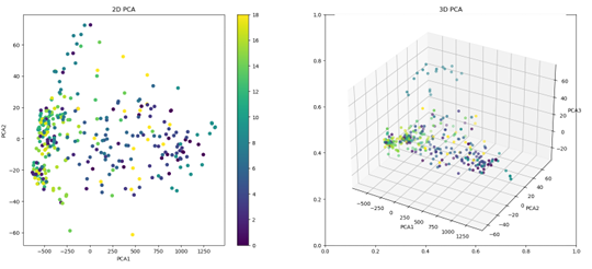
Self Label weights for ResNet50
0.12, while the entropy ranged from 0.00 to 0.12, as shown in Figure 3.18.
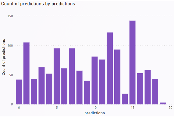
The confidence of the semantic clusters for each class can be seen in Figure 3.22. This image outlines the confidence probability of classification for each generated image. It was found that in general, minus classification 7, that our conditional GAN
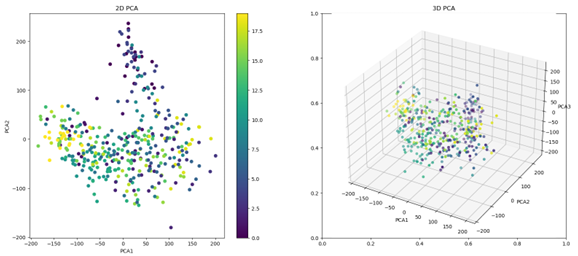
using (SCAN) weights for ResNet50
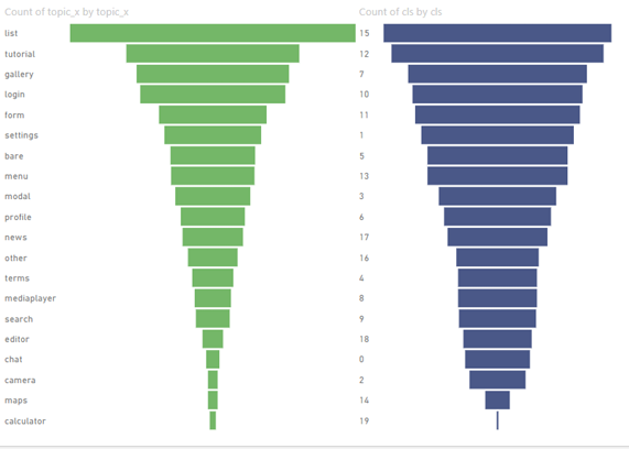
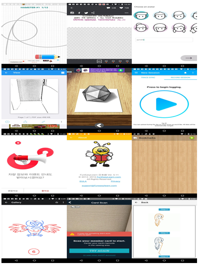
is fairly confident on its chosen image classifications. See in Figure 3.20, the models distribution of the RICO images resembles that of the manually labeled enRICO dataset. For example if we pull samples from cluster 15 we can expect to find images relating to UI lists 3.21.
using Self Label weights for ResNet50
Ourclustering models demonstrate the effectiveness of using unsupervised learning techniques to cluster UI images based on their visual similarity. Our analysis shows that the performance of our models is largely dependent on the quality and quantity of training data, as well as the effectiveness of the feature extraction and clustering algorithms. However, it can be seen as we continue to train our clustering models that our generated images clusters continue to get further apart. Signalling precision and diversity in our GAN. Despite the challenges posed by limited and unannotated data, our models have shown promising results in accurately clustering UI layouts and assessing the performance of the Generative Adversarial Network.
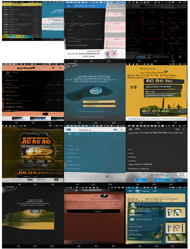
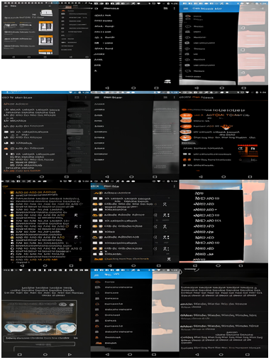
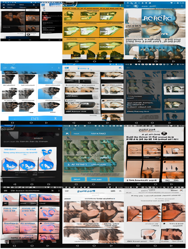
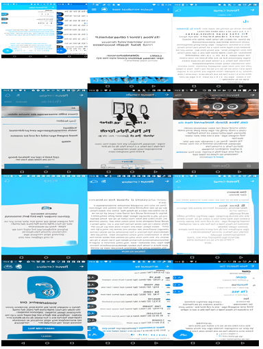
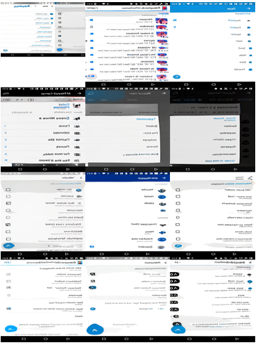
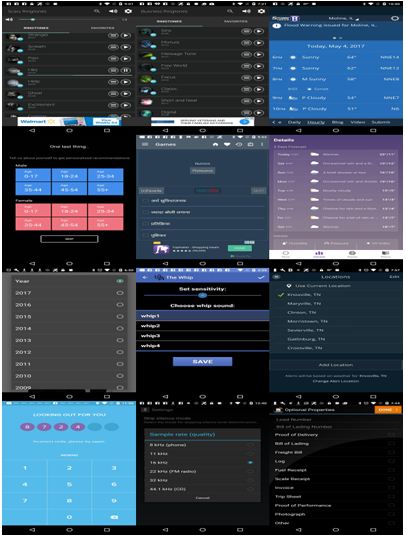
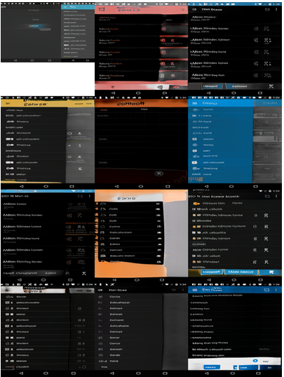
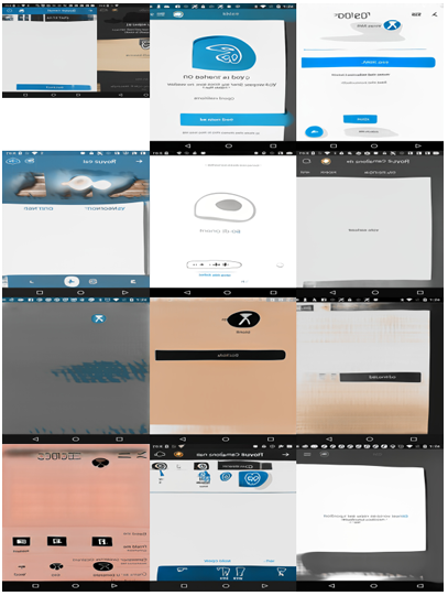
The images located in Appendix A were randomly selected from our generated images based on cluster. Notice the quality of the generative model at FID score 12.74 as well as the similarity between images in the clusters. Additionally in Appendix A you can view the image similarity of the clusters of top 12 RICO images. Here in Figures 3.23, 3.25, 3.27 and 3.24, 3.26, 3.24you can see the generated and top images
found to be the best sampled starting point for RICO image clustering.
for cluster 0-2.
The remaining part of the results section, including the top 12 RICO classifications for Clusters 3-19, can be found in Appendix B. The top 12 classifications for Cluster 0 are presented in Figure 3.23. Overall, the top-12 images for each of the classifications share similar features, such as screen geometric distribution, advertisement markings, lists, and sections. Appendix B also includes 12 randomly sampled GAN image generations that have been classified into classifications 1-19 without ground truth labels. The top 12 classifications for Cluster 0 using images from the conditional GAN trained on RICO image data are presented in Figure 3.24.
3.3 Showcasing the Conditional GAN Results
In the training of the Siamese neural network, as described in Section 2.4 and detailed in Section 2, the anchor-negative pairs were selected at random from the image class with the least similarity. Knowing dissimilar image classifications helps solve the objective function to minimize the distance between known positive images while maximizing the distance from known negatives. To address this, we calculated the Euclidean distance between each of the top 12 most confident samples from each of
the 20 semantic clusters, the results can be seen in Appendix A.
The Siamese Network Architecture defined later in this section displays the architecture for this researches Siamese network, which is used to generate conditional GAN images as part of our research. The network takes in three input layers for anchor, positive, and negative images, respectively. The pretrained ResNet50 model is used for feature extraction, and dropout layers are added to prevent overfitting.
The output is then reduced to a 512-dimensional feature vector, which is used in the distance layer to calculate the similarity between pairs of images. Finally, the Siamese network is compiled using the triplet loss function described in Section 2.4 and the Adam optimizer.
Our Siamese Architecture can be seen in code Siamese Network Architecture.
Table 3.1: Classification Results
Classification Least Similar Class 00 Least Similar Class 01 Least Similar Class 02
0 11 12 10
1 9 4 0
2 9 4 0
3 11 12 10
4 11 12 10
5 11 17 12
6 11 12 10
7 9 4 0
8 9 4 0
9 11 12 10
10 9 4 0
11 9 4 0
12 9 4 0
13 9 4 0
14 9 4 0
15 9 4 0
16 9 4 0
17 9 4 0
18 11 12 10
19 11 12 10
of Classifications of Generated Images
During the training process, we used approximately 1,000 sketch-image pairs, and we performed hyper-parameter tuning on each epoch batch. Our results indicated that using a larger number of images over a shorter number of epoch intervals improved s the accuracy of the model, while training extensively over a smaller number of images led to mode collapse. The Siamese network was trained for 8 epochs, with each epoch consisting of 125 images. The total loss progressively decreased towards 0, with the training set showing a loss of 26.17 and the validation set showing a loss of 0.55 at the end of epoch 1 of 8. By the end of epoch 3, the testing loss was reduced to 0.06, with validation at 0.08. We completed the Siamese training with triplet loss, which resulted in a training set loss of 0.033 and a validation set loss of 0.075. Continued
training beyond epoch 8 led to mode collapse.
To evaluate the distance between each of the sketch-image pairs, we compared the distance between a positive anchor pair and all other anchor negative pairs using

four distance metrics: Euclidean, Cosine, Infinity, Manhattan, and Hamming. The evaluation for these metrics lasted for 25 hours and 26 minutes. We determined that for our image set, Euclidean distance was the most effective in terms of image distance similarity.
The average anchor positive score for Euclidean distance was 0.067, with Cosine
Similarity at 0.113, Infinity Metric at 0.114, Manhattan at 0.074, and Hamming
at 0.100.
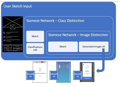
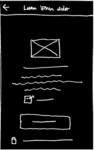
In solving the image-to-image problem, view Figure 3.29 Research Question 3, we used the top 12 most confidently classified generated GAN images from the trained semantic clustering model. We input a user’s sketch into the Siamese network to compare it to the 20 different UI classifications, resulting in a total of 240 distance calculations.
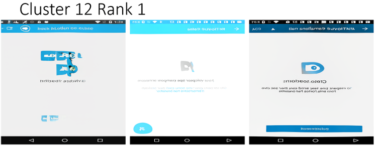
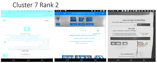
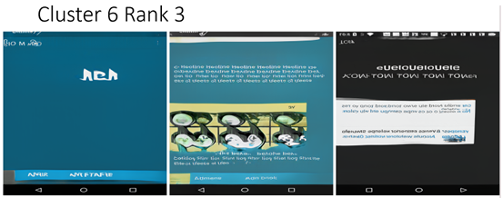
We calculated the average distance from each classification and selected the top three closest image representations as the sketch classification. Due to the interpretative nature of freehand sketches, we selected the top three classifications and images to account for discrepancies in the possible interpretations of a user’s sketch. The resulting images generated from multiple possible classifications have the potential to provide a broader range of valuable images. Figure 3.30 shows an example of a user’s sketch, and Figures 3.31, 3.32, and 3.33 depict the top returned
cluster-generated images from the trained Siamese network.
Listing 3.1: Siamese Network Architecture
input layers
anchor = Input(shape=(224, 224, 3), name=’anchor’)
positive = Input(shape=(224, 224, 3), name=’positive’)
negative = Input(shape=(224, 224, 3), name=’negative’)
# Load pre-trained ResNet50
resnet = ResNet50(weights=SELFLABEL,
include_top=False,
input_shape=(224, 224, 3))
# Define feature extraction layers
x = resnet(anchor)
x = resnet(positive)
x = resnet(negative)
# Add dropout layers
x = Dropout(0.5)(x)
x = Dropout(0.5)(x)
x = Dropout(0.5)(x)
# Reduce to 512-dimensional feature vectors
x = Dense(512, activation=’relu’, name=’reduce’)(x)
# Define distance layer
distance_layer = DistanceLayer()([x, x, x])
# Define siamese network
siamese_network = Model(inputs=
[anchor, positive, negative],
outputs=distance_layer)
# Compile model
siamese_network.compile(loss=triplet_loss, optimizer=’adam’)

CHAPTER 4
DISCUSSION
In this study, the proposed approach for generating UI designs using a Conditional GAN and Semantic Clustering showed promising results. The generated UI designs were diverse and resembled real-world UI designs. The Siamese network, used for image-to-image comparison, provided an accurate classification of the user input sketch. The use of semantic clustering for training the Conditional GAN allowed for generating images on multiple possible classifications, resulting in a broader range of valuable images returned.
Section 2.2 in Chapter 2 outlined FID score and Section 3.1 in Chapter 3 presented that a GAN with limited training data can generate realistic UI layout images, measured by the FID Score. Effectively answering research question one, ”Can a GANwith limited training data generate realistic UI layout images, measured by the FID Score?”
Section 2.3 in Chapter 2 outlined Semantic Clustering and Section 3.2 in Chapter 3 presented that we can cluster GAN-generated UI layouts when trained on limited image data with no ground truth image classifications. However the accuracy of these classifications are low. Manually evaluating the image clusters shows overall similarity of each found cluster classification. This Answers research question two, ”How accurately can we cluster GAN-generated UI layouts when trained on limited image data with no ground truth image classifications?”.
The study showed that the use of the triplet loss function resulted in a significant improvement in the performance of the Siamese network. By using the top 12 most confident classified generated GAN images from the trained semantic clustering model, the Siamese network could cross-compare between the 20 different UI clas sifications, resulting in accurate classification of the user input sketch. However, it was found that training the Siamese network extensively over fewer images led to mode collapse, which is a common problem in GAN-based models.
This suggests that careful hyperparameter tuning and monitoring of the model’s training progress
is important to achieve optimal performance. In terms of evaluating the distance metric between the generated images and the user input sketch, it was found that the Euclidean distance was the most effective measure for determining image distance similarity. This is an important finding, as it suggests that the Euclidean distance is a good choice for measuring the similarity between sketches and images, and can be used to improve the accuracy of the Con ditional GAN and Semantic Clustering approach.
This and Section 2.4 in Chapter 2 and Section 3.3 in Chapter 3, answers research question three, ”How can a conditional GAN train on no labeled image data map a user’s input sketch to a generated UI layout?”.
While the returned generated images were within proper bounds of similarity, there are still areas for improvement in our approach. For instance, incorporating feature vectors of the previous two models as input for the Siamese network could have significantly improved its ability to discover the true image-to-image distance. Additionally, there was found to be an error in computing accuracy. It was misunderstood during the testing process that giving enRICO labels 0-19 would line up with the clustering models 0-19 classifications. A novice mistake, had the human labeled classifications been evaluated to line up with the labels of the classifiers clusters, the accuracy of the clusters could of appeared at a much higher percentage.
Nonetheless, our research has demonstrated that a conditional GAN can be created to solve image-to-image translation problems without domain knowledge of the images and a large labeled image set. This framework has the potential to facilitate experimentation with different image-to-image problems for developers and users. Moreover, while our approach does not have the capability to measure the confidence of GAN generated clustered images, human observers can observe the labeled classifications in the clusters to gain a better understanding of their relatedness. This research would of benefited from displaying the feature vectors in latent space of all RICO and Generated Images. Along with their sketch counterparts from the Siamese network.
Despite promising results, there are several limitations to this study. Firstly, the dataset used in this study was limited to UI designs from a single source, which may not be representative of all possible UI designs. Secondly, the proposed approach requires a significant amount of computational power to generate a single UI design. Therefore, further research is needed to optimize the performance of the proposed approach to make it more feasible for real-world applications.
In future work, the proposed approach can be extended to incorporate user feed back in the generation process. By allowing users to provide feedback on the generated designs, the Conditional GAN and Semantic Clustering approach can be further improved. Additionally, the proposed approach can be used to generate UI designs in different styles, such as flat design or material design. Overall, the proposed approach has the potential to revolutionize the UI design process by providing a faster and more efficient way of generating high-quality UI designs.
REFERENCES
[1] Chun-Chen Chang, Yen-Yu Liu, and Yung-Yu Chuang. Guided image synthesis with reconfigurable references. arXiv preprint arXiv:2007.14797, 2020.
[2] Sumit Chopra, Raia Hadsell, and Yann LeCun. Learning a similarity metric discriminatively, with application to face verification. In 2005 IEEE Computer Society Conference on Computer Vision and Pattern Recognition (CVPR’05), volume 1, pages 539–546. IEEE, 2005.
[3] Bhaskar Deka, Jerry Cao, Heng Gao, Paul Jenkins, Yash Turakhia, Zachary Wartell, and Zijian Zhang. Rico: A mobile app dataset for building data-driven design applications. In Proceedings of the 2017 CHI Conference on Human Factors in Computing Systems, pages 4186–4197. ACM, 2017.
[4] Arnab Ghosh, Richard Zhang, Puneet K. Dokania, Oliver Wang, Alexei A. Efros, Philip H. S. Torr, and Eli Shechtman. Interactive sketch & fill: Multiclass sketch to-image translation. pages 1171–1180.
[5] Ian J. Goodfellow, Jean Pouget-Abadie, Mehdi Mirza, Bing Xu, David Warde Farley, Sherjil Ozair, Aaron Courville, and Yoshua Bengio. Generative adversarial networks, 2014.
[6] David Ha and Douglas Eck. A neural representation of sketch drawings.
[7] Viet Khanh Ha, Jinchang Ren, Xinying Xu, Sophia Zhao, Gang Xie, and Valentin Masero Vargas. Deep learning based single image super-resolution: A survey. In Advances in Brain Inspired Cognitive Systems: 9th International Conference, BICS 2018, Xi’an, China, July 7-8, 2018, Proceedings 9, pages 106–119. Springer, 2018.
[8] Forrest Huang and John F. Canny. Sketchforme: Composing sketched scenes from text descriptions for interactive applications.
[9] Forrest Huang, Eldon Schoop, David Ha, and John Canny. Scones: Towards conversational authoring of sketches. pages 313–323.
[10] Hongxun Huang, Zhixin Liu, Tong Zhang, Hanbin Fang, and Jian Sun. High-fidelity and occlusion-aware face swapping with cs-gan. arXiv preprint arXiv:2009.01091, 2020.
[11] Xun Huang and Serge Belongie. Arbitrary style transfer in real-time with adaptive instance normalization. In Proceedings of the IEEE International Conference on Computer Vision, pages 1501–1510, 2017.
[12] Zifeng Huang. Deep-learning-based machine understanding of sketches: Recognizing and generating sketches with deep neural networks | EECS at UC berkeley.
[13] Tero Karras, Samuli Laine, and Timo Aila. A style-based generator architecture for generative adversarial networks. In Proceedings of the IEEE Conference on Computer Vision and Pattern Recognition, pages 4401–4410, 2019.
[14] Tero Karras, Samuli Laine, and Timo Aila. Analyzing and improving the image quality of stylegan. In Proceedings of the IEEE/CVF Conference on Computer Vision and Pattern Recognition, pages 8110–8119, 2020.
[15] Gregory Koch, Richard Zemel, and Ruslan Salakhutdinov. Siamese neural networks for one-shot image recognition. In ICML deep learning workshop, volume 2, pages 1–8, 2015.
[16] Mark Lee, Saining Xie, Patrick Gallagher, and Zhuowen Zhang. Mobilenetv2: Inverted residuals and linear bottlenecks. Proceedings of the IEEE Conference on Computer Vision and Pattern Recognition, pages 4510–4520, 2019.
[17] Luis A. Leiva, Asutosh Hota, and Antti Oulasvirta. Enrico: A high-quality dataset for topic modeling of mobile UI designs. In Proc. MobileHCI Adjunct, 2020.
[18] Lingzhi Li, Jianmin Bao, Hao Yang, Dong Chen, and Fang Wen. Faceshifter: Towards high fidelity and occlusion aware face swapping, 2019.
[19] Rui Li, Qianfen Jiao, Wenming Cao, Hau-San Wong, and Si Wu. Model adaptation: Unsupervised domain adaptation without source data. In Proceedings of the IEEE/CVF Conference on Computer Vision and Pattern Recognition (CVPR), June 2020.
[20] Mehdi Mirza and Simon Osindero. Conditional generative adversarial nets. In Advances in neural information processing systems, pages 2672–2680, 2014.
[21] Augustus Odena, Christopher Olah, and Jonathon Shlens. Conditional image synthesis with auxiliary classifier gans. In International Conference on Machine Learning, pages 2642–2651, 2017.
[22] Changhoon Oh, Jungwoo Song, Jinhan Choi, Seonghyeon Kim, Sungwoo Lee, and Bongwon Suh. I lead, you help but only with enough details: Understanding user experience of co-creation with artificial intelligence. In Proceedings of the 2018 CHI Conference on Human Factors in Computing Systems, pages 1–13. Association for Computing Machinery.
[23] Florian Schroff, Dmitry Kalenichenko, and James Philbin. FaceNet: A unified embedding for face recognition and clustering. pages 815–823. ISSN: 1063-6919.
[24] Yujun Shen, Jiaying Liu, and Ling Shao. Controllable stylegan2: Improved expression control in generative face models. arXiv preprint arXiv:2104.13426, 2021.
[25] Yujun Shen, Jiaying Liu, and Ling Shao. Unsupervised domain adaptation with conditional stylegan2. arXiv preprint arXiv:2101.05276, 2021.
[26] Xinxiao Tao, Xiaolong Li, Peixiang Li, and Rui Xu. Gan-based data augmentation for mobile ui design. In 2020 IEEE International Conference on Systems, Man, and Cybernetics (SMC), pages 4038–4043. IEEE, 2020.
[27] Wouter Van Gansbeke, Simon Vandenhende, Stamatios Georgoulis, Marc Proesmans, and Luc Van Gool. Scan: Learning to classify images without labels. In European Conference on Computer Vision, pages 268–285. Springer, 2020.
[28] Jiacheng Xu, Xingyu Zhao, Peng Zhang, and Jun Wang. Strotss: Unsupervised spatial transformations for self-supervised learning. arXiv preprint arXiv:2101.06740, 2021.
[29] Han Zhang, Tao Xu, Hongsheng Li, Shaoting Zhang, Xiaogang Wang, Xiaolei Huang, and Dimitris N. Metaxas. StackGAN: Text to photo-realistic image synthesis with stacked generative adversarial networks. pages 5907–5915.
[30] Yang Zhao, Xiaolong Wang, Xiaolong Wu, Zheng Zhang, and Yanwei Fu. Scenegan: Scene-consistent text-to-image generation with transformers. arXiv preprint arXiv:2103.01209, 2021.
APPENDIX A
MODEL PARAMETERS
A.1 Pretext Model Training Parameters
{’setup’: ’moco’,
’backbone’: ’resnet50’,
’model_kwargs’:
{’head’: ’mlp’,
’features_dim’: 128},
’train_db_name’: ’rico-20’,
’val_db_name’: ’rico-20’,
’num_classes’: 20,
’temperature’: 0.07,
’batch_size’: 128,
’num_workers’: 8,
’transformation_kwargs’:
{’crop_size’: 224,
’normalize’:
{’mean’: [0.485, 0.456, 0.406],
’std’: [0.229, 0.224, 0.225]}}}
A.2 Semantic Clustering Model Training Parameters
{’setup’: ’scan’,
’criterion’: ’scan’,
’criterion_kwargs’: {’entropy_weight’: 5.0},
’backbone’: ’resnet50’,
’update_cluster_head_only’: True,
’num_heads’: 10,
’train_db_name’: ’rico-20’,
’val_db_name’: ’rico-20’,
’num_classes’: 20,
’num_neighbors’: 20,
’augmentation_strategy’: ’simclr’,
’augmentation_kwargs’: {
’random_resized_crop’: {’size’: 224,
’scale’: [0.2, 1.0]},
’color_jitter_random_apply’: {’p’: 0.8},
’color_jitter’: {’brightness’: 0.4,
’contrast’: 0.4,
’saturation’: 0.4,
’hue’: 0.1},
’random_grayscale’: {’p’: 0.2},
’normalize’: {’mean’: [0.485, 0.456, 0.406],
’std’: [0.229, 0.224, 0.225]}},
’transformation_kwargs’: {’crop_size’: 224,
’normalize’: {’mean’: [0.485, 0.456, 0.406],
’std’: [0.229, 0.224, 0.225]}},
’optimizer’: ’sgd’,
’optimizer_kwargs’: {’lr’: 5.0,
’weight_decay’: 0.0,
’nesterov’: False,
’momentum’: 0.9},
’epochs’: 100,
’batch_size’: 512,
’num_workers’: 12,
’scheduler’: ’constant’}
A.3 Self-Labeling Model Training Parameters
{’setup’: ’selflabel’,
’confidence_threshold’: 0.99,
’use_ema’: True,
’ema_alpha’: 0.999,
’criterion’: ’confidence-cross-entropy’,
’criterion_kwargs’: {’apply_class_balancing’: False},
’backbone’: ’resnet50’,
’num_heads’: 1,
’train_db_name’: ’rico-20’,
’val_db_name’: ’rico-20’,
’num_classes’: 20,
’augmentation_strategy’: ’ours’,
’augmentation_kwargs’:
{’crop_size’: 224,
’normalize’:
{’mean’: [0.485, 0.456, 0.406],
’std’: [0.229, 0.224, 0.225]},
’num_strong_augs’: 4,
’cutout_kwargs’:
{’n_holes’: 1,
’length’: 75,
’random’: True}},
’transformation_kwargs’:
{’crop_size’: 224,
’normalize’:
{’mean’: [0.485, 0.456, 0.406],
’std’: [0.229, 0.224, 0.225]}},
’optimizer’: ’sgd’,
’optimizer_kwargs’:
{’lr’: 0.03,
’weight_decay’: 0.0,
’nesterov’: False,
’momentum’: 0.9},
’epochs’: 75,
’batch_size’: 128,
’num_workers’: 16,
’scheduler’: ’constant’}
A.4 Generative Adversarial Training Network
Load ingtrainingset…
Num images:132522
Image shape:[3,512,512]
Label shape:[0]
Constructing networks…
Resuming from
“/bsuhome/hkiesecker/scratch/styleGAN/RICO1024_Trained_Auto_512/00000-RICO512x512-mirror
Setting up Py Torch plugin”bias_act_plugin”…Done.
Setting up Py Torchplugin”up firdn2d_plugin”…Done.
Generator Parameters Buffers Out put shape Datatype————–
mapping.fc0 262656 – [8,512] float 32
mapping.fc1 262656 – [8,512] float 32
mapping – 512 [8,16,512] float 32
synthesis.b4.conv1 2622465 32 [8,512,4,4] float 32
synthesis.b4.torgb 264195 – [8,3,4,4] float 32
synthesis.b4:0 8192 16 [8,512,4,4] float 32
synthesis.b4:1 – – [ 8,512,4,4] float 32
synthesis.b8.conv0 2622465 80 [8,512,8,8] float 32
synthesis.b8.conv1 2622465 80 [8,512,8,8] float 32
synthesis.b8.torgb 264195 – [8,3,8,8] float 32
synthesis.b8:0 – 16 [8,512,8,8] float 32
synthesis.b8:1 – – [8,512,8,8] float 32
synthesis.b16.conv02622465 272 [8,512,16,16] float 32
synthesis.b16.conv12622465 272 [8,512,16,16] float 32
synthesis.b16.torgb264195- [8,3,16,16] float 32
synthesis.b16:0 – 16 [8,512,16,16] float 32
synthesis.b16:1 – – [8,512,16,16] float 32
synthesis.b32.conv02622465 1040 [8,512,32,32] float 32
synthesis.b32.conv12622465 1040 [8,512,32,32] float 32
synthesis.b32.torgb264195 – [8,3,32,32] float 32
synthesis.b32:0 – 16 [8,512,32,32] float 32
synthesis.b32:1 – – [8,512,32,32] float 32
synthesis.b64.conv02622465 4112 [8,512,64,64] float 16
synthesis.b64.conv12622465 4112 [8,512,64,64] float 16
synthesis.b64.torgb264195 – [8,3,64,64] float 16
synthesis.b64:0 – 16 [8,512,64,64] float 16
synthesis.b64:1 — [8,512,64,64] float 32
synthesis.b128.conv01442561 16400 [8,256,128,128] float 16
synthesis.b128.conv1721409 16400 [8,256,128,128] float 16
synthesis.b128.torgb132099 – [8,3,128,128] float 16
synthesis.b128:0 – 16 [8,256,128,128] float 16
synthesis.b128:1 – – [8,256,128,128] float 32
synthesis.b256.conv0426369 65552 [8,128,256,256] float 16
synthesis.b256.conv1213249 65552 [8,128,256,256] float 16
synthesis.b256.torgb66051 – [8,3,256,256] float 16
synthesis.b256:0 – 16 [8,128,256,256] float 16
synthesis.b256:1 – – [8,128,256,256] float 32
synthesis.b512.conv0 139457 262160 [8,64,512,512] float 16
synthesis.b512.conv1 69761 262160 [8,64,512,512] float 16
synthesis.b512.torgb 33027- [8,3,512,512] float 16
synthesis.b512:0 – 16 [8,64,512,512] float 16
synthesis.b512:1 — [8,64,512,512]float 32————–
Total 28700647 699904 – –
Discriminator Parameters Buffers Out put shape Datatype
b512.fromrgb 256 16 [8,64,512,512] float 16
b512.skip 8192 16 [8,128,256,256] float 16
b512.conv0 36928 16 [8,64,512,512] float 16
b512. conv 1 73856 16 [8,128,256,256] float 16
b5 12 – 16 [8,128,256,256] float 16
b25 6. skip 32768 16 [8,256,128,128] float 16
b256.conv0 147584 16 [8,128,256,256] float 16
b256.conv1 295168 16 [8,256,128,128] float 16
b256 – 16 [8,256,128,128] float 16
b128.skip 131072 16 [8,512,64,64] float 16
b128.conv0 590080 16 [8,256,128,128] float 16
b128.conv1 1180160 16 [8,512,64,64] float 16
b128 – 16 [8,512,64,64] float 16
b64.skip 262144 16 [8,512,32,32] float 16
b64.conv0 2359808 16 [8,512,64,64] float 16
b64.conv1 2359808 16 [8,512,32,32] float 16
b64 – 16 [8,512,32,32] float 16
b32.skip 262144 16 [8,512,16,16] float 32
b32.conv0 2359808 16 [8,512,32,32] float 32
b32.conv1 2359808 16 [8,512,16,16] float 32
b32 – 16 [8,512,16,16] float 32
b16.skip 262144 16 [8,512,8,8] float 32
b16.conv0 2359808 16 [8,512,16,16] float 32
b16.conv1 2359808 16 [8,512,8,8] float 32
b16 – 16 [8,512,8,8] float 32
b8.skip 262144 16 [8,512,4,4] float 32
b8.conv0 2359808 16 [8,512,8,8] float 32
b8.conv1 2359808 16 [8,512,4,4] float 32
b8 – 16 [8,512,4,4] float 32
b4.mbstd – – [8,513,4,4] float 32
b4.conv 2364416 16 [8,512,4,4] float 32
b4.fc 4194816 – [8,512] float 32
b4.out 513- [8,1] float 32
—– —— — —- —- —– —- —-
Total 28982849 480 – –
Setting up augmentation…
Distributing a cross4 G P Us…
Setting up training phases…
Exporting sample images…
Initializing logs…
Training for 25000 kimg…
APPENDIX B
REFERENCE IMAGES FOR RESULTS CHAPTER
Validation RICO images Top 12 Confident Samples for Clusters 1-19 and Randomly Sampled Generated UI Images from Trained GAN for Clusters 1-19.
