Excel’s MAP function is genius

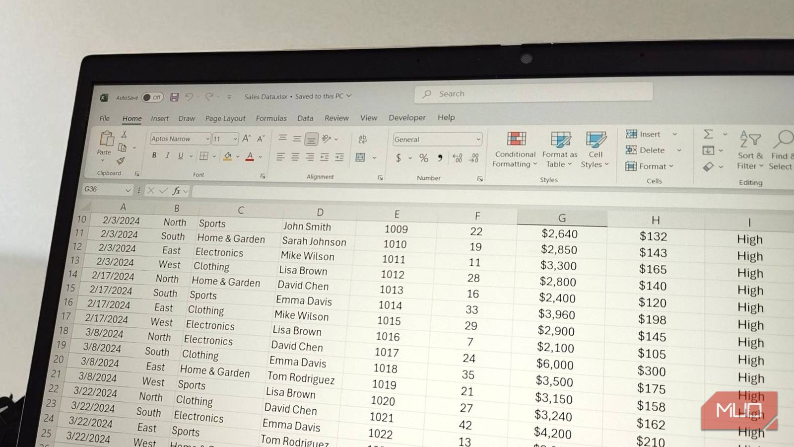
If you’ve ever found yourself copying the same formula down hundreds of rows in Excel, you know how tedious it gets. The usual approach, dragging formulas, adjusting cell references, and hoping nothing breaks, works, but it’s far from efficient. Excel’s MAP function changes that. Instead of applying formulas one cell at a time, MAP processes entire ranges of data at once, to make your Excel spreadsheets cleaner and your workflow faster.

It’s not about reorganizing everything you do, but it’s a smarter way to handle repetitive tasks. Therefore, MAP is worth exploring if you’re still relying on traditional formulas for array operations.

How does the MAP function work?

MAP and its partner, LAMBDA, work together

The MAP function takes a range of data and applies a custom calculation to the entire dataset in one go. It uses the following syntax:

=MAP(array, lambda)

Let’s break down the parameters:

• array: This is the range of cells you want to process. It can be a single column, multiple columns, or even an entire table. MAP will loop through each value in this range.
• lambda: This is where you define the calculation. Think of it as a mini-formula that tells MAP what to do with each value. You create it using Excel’s LAMBDA function, which lets you write formulas like a human with custom logic without repeating formulas.

When you run MAP, it applies your lambda function to every cell in the array and returns a new set of results. The output matches the size and shape of your input, so if you feed it 10 rows, you get 10 results back.

What makes MAP different from traditional formulas is that it doesn’t rely on cell references that shift as you copy. The logic stays locked inside the function, so there’s no risk of accidentally breaking a formula when you move things around.

Start with a simple task to see MAP in action

Let’s add markup to product prices with one formula

Credit: Yasir Mahmood /

Let’s say you have a list of product prices and need to add a 10% markup to each one. The traditional way would be to write a formula like =B2*1.1 and drag it down. However, MAP handles this differently.

Instead of writing individual formulas, you create one MAP function that processes the entire price column:

=MAP(B2:B11, LAMBDA(price, price*1.1))

Here’s what happens: MAP takes each value in B2:B11 (your price range) and feeds it into the LAMBDA function. The LAMBDA assigns each value to the variable “price”, multiplies it by 1.1, and returns the result. All in one step.

The benefit here is that you’re not creating multiple formulas, and if your data changes, the MAP function recalculates automatically.

You can name your LAMBDA variable anything you want. I used “price” because it’s clear, but “p” or “x” would work just as well. The variable is just a placeholder that represents each value as MAP processes the array.

Let’s add more logic to MAP with the IF statement

You can nest other functions

Credit: Yasir Mahmood /

MAP isn’t limited to simple calculations. You can add Excel conditional functions inside the LAMBDA function to handle different scenarios based on the data.

Let’s say you want to apply different markup rates depending on the price. Products $100 or more get a 10% markup, while products below that get a 15% markup. Here’s how you’d write that:

=MAP(B2:B11, LAMBDA(price, IF(price>=100, price*1.1, price*1.15)))

The IF statement checks each price as MAP processes it. If the price is $100 or more, it multiplies by 1.1. Otherwise, it multiplies by 1.15.

You can stack even more conditions if needed. If you want to add tax calculations, apply tiered discounts, or round to specific decimal places, just build the logic into your LAMBDA function. MAP will apply it to every value in the array.

MAP handles multiple columns and messy text data

Let’s standardize a list of names with a single formula

Credit: Yasir Mahmood /

MAP isn’t restricted to single-column operations. You can feed it multiple arrays and process them together in one function.

Say you want to calculate total sales by multiplying price and quantity. Instead of creating a separate formula column, use MAP to handle both:

=MAP(B2:B11, C2:C11, LAMBDA(price, qty, price*qty))

MAP takes two arrays—B2:B11 (prices) and C2:C11 (quantities)—and processes them row by row. The LAMBDA function receives both values, multiplies them, and returns the result.

You can also use MAP to clean up text data. If your product names are inconsistent—some in all caps, others in lowercase, or filled with extra spaces—you can easily standardize everything at once:

=MAP(A2:A11, LAMBDA(text, PROPER(TRIM(text))))

This formula trims unnecessary spaces and converts each product name to the proper case. TRIM removes leading and trailing spaces, while PROPER capitalizes the first letter of each word. MAP applies both functions to every cell in the range simultaneously.

Credit: Yasir Mahmood /

MAP is just the beginning

Expand your Excel toolkit

Once you’re comfortable with MAP, you’ll find it easier to pick up other LAMBDA helper functions like REDUCE, SCAN, and BYROW/BYCOL. They all work on the same principle—processing arrays with custom logic instead of dragging formulas.

The advantage isn’t just speed. It’s about building spreadsheets that are easier to maintain. When your logic lives inside a single function, you can update it once and see changes everywhere. I recommend starting with simple tasks, such as markups, basic calculations, and text cleanup. Once MAP clicks, you’ll spot opportunities to use it everywhere.