How Stylised Facts Shape the Future of Financial Market Simulation | HackerNoon

Table of Links

Abstract, Acknowledgements, and Statements and Declarations

1. Introduction

2. Background and Related Work

   2.1 Agent-based Financial Market simulation

   2.2 Flash Crash Episodes

3. Model Structure and 3.1 Model Set-up

   3.2 Common Trader Behaviours

   3.3 Fundamental Trader (FT)

   3.4 Momentum Trader (MT)

   3.5 Noise Trader (NT)

   3.6 Market Maker (MM)

   3.7 Simulation Dynamics

4. Model Calibration and Validation and 4.1 Calibration Target: Data and Stylised Facts for Realistic Simulation

   4.2 Calibration Workflow and Results

   4.3 Model Validation

5. 2010 Flash Crash Scenarios and 5.1 Simulating Historical Flash Crash

   5.2 Flash Crash Under Different Conditions

6. Mini Flash Crash Scenarios and 6.1 Introduction of Spiking Trader (ST)

   6.2 Mini Flash Crash Analysis

   6.3 Conditions for Mini Flash Crash Scenarios

7. Conclusion and Future Work

   7.1 Summary of Achievements

   7.2 Future Works

References and Appendices

4 Model Calibration and Validation

In this section we present the methodology for calibrating the agent-based financial market. Calibration means finding an optimal set of model parameters to make the model generate the most realistic simulated financial market. Firstly we describe the real data and the associated stylised facts in financial markets. Next we define the distance between historical and simulated stylised facts, which acts as the loss function in the calibration process. The parameters calibration workflow is presented, followed by detailed validation of the proposed high-frequency financial market simulator.

4.1 Calibration Target: Data and Stylised Facts for Realistic Simulation

In the model calibration process, real financial market data is essential for setting up the calibration target. We collected high-frequency limit order book data of E-mini S&P 500 futures, from May 3rd, 2010 to May 6th, 2010[7]. We select the most liquid contract as the calibration target, which is the contract expires in June 2010. Our dataset comprises high-frequency information for 10 levels of limit order book update, both the buy side and sell side.

Financial price time series data display some interesting statistical characteristics that are commonly called stylised facts. According to Sewell (2011), stylized facts refer to empirical findings that are so consistent (for example, across a wide range of financial instruments and different time periods) that they are accepted as truth. A stylized fact is a simplified presentation of an empirical finding in financial markets. A successful and realistic financial market simulation is capable of reproducing various stylised facts. These stylised facts include fat-tailed distribution of returns, autocorrelation of returns, and volatility clustering. The loss function used in the calibration process is constructed by measuring the distance between historical and simulated stylised facts.

4.1.1 Fat-tailed distribution of returns

The distributions of price returns have been found to be fat-tailed across all timescales. In other words, the return distributions exhibit positive excess kurtosis. Understanding positively kurtotic return distributions is important for risk management since large price movements are much more likely to occur than in commonly assumed normal distributions.

Following the convention in literature, in this paper we investigate the stylised fact of fat-tailed returns by examining second-level intra-day price returns. Both millisecond-level historical and simulated mid-price time series are resampled into second-level frequency and we examine the mid-price returns for each second. Specifically, the last price snapshot is taken as the price for that specific second. Second-level price returns are calculated accordingly. Our experiments show that different time scales have no significant influence on the final results. The main metric used for evaluating the fat-tail characteristic is the Hill Estimator of the tail index (Hill 2010). A lower value of the Hill Estimator implies that the return distribution has a fatter tail.

4.1.2 Autocorrelation of returns

Autocorrelation is defined to be a mathematical representation of the degree of similarity between a time series and a lagged version of the same time series. It measures the relationship between a variable’s past values and its current value. Take first-order autocorrelation for example. A positive first-order autocorrelation of returns indicates that a positive (negative) return in one period is prone to be followed by a positive (negative) return in the subsequent period. Instead, if the first-order autocorrelation of returns is negative, a positive (negative) return will usually be followed by a negative (positive) return in the next period. It is observed that the returns series lack significant autocorrelation, except for weak, negative autocorrelation on very short timescales. McGroarty et al. (2019) show that the negative autocorrelation of returns is significantly stronger at a smaller time horizon and disappears at a longer time horizon. Examination of our data also reveals this stylised fact. Figure 1 shows the autocorrelation function of second-level return time series for E-mini S&P 500 futures on two days. We can see that the autocorrelation is significantly negative for very small lags, and the negative autocorrelation gradually disappears for larger lags.

4.1.3 Volatility clustering

Financial price returns often exhibit the volatility clustering property: large changes in prices tend to be followed by large changes, while small changes in prices tend to be followed by small changes. This property results in the persistence of the amplitudes of price changes (Cont 2007). It is found that the volatility clustering property exists on timescales varying from minutes to days and weeks. Volatility clustering also refers to the long memory of square price returns (McGroarty et al. 2019). Consequently, volatility clustering can be manifested by the slow decaying pattern in the autocorrelation of squared returns. Specifically, for short lags the autocorrelation function of squared returns is significantly positive, and the autocorrelation slowly decays with the lags increasing. Figure 2 shows the autocorrelation patterns for squared second-level returns for E-mini S&P 500 futures on two days. It is shown that the volatility clustering stylised fact clearly exists in our collected E-mini S&P 500 futures price dataset.

4.1.4 Stylised Facts Distance as Loss Function

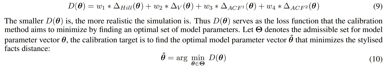
The target for agent-based model calibration is to find an optimal set of model parameters to make the model generate a realistic simulated financial market. To solve this optimization problem, it is essential to have a metric that is able to quantify the “realism” of a simulated financial market. First of all, a realistic simulated financial market must exhibit similar characteristics to real financial markets, such as the fat-tailed return distribution and volatility level. In addition, realistic simulated financial data are also required to reproduce other stylised facts such as the autocorrelation patterns in returns and squared returns. Here we design a stylised facts distance to quantify the similarities between simulated and historical financial data. Four metrics are considered in the stylised facts distance: Hill Estimator of the tail index for absolute return distributions, volatility, autocorrelation of returns and autocorrelation of squared returns. For each metric, the differential quantity between simulated value and historical value is calculated. The stylised facts distance is then calculated as the weighted sum of the four differential quantities:

Detailed calculations of the four quantities in the stylised facts distance are presented below.

The Hill Estimator is famous for inferring the power behaviour in tails of experimental distribution functions. Following Franke and Westerhoff (2012), we use the Hill Estimator of the tail index to estimate the degree of fat-tail in the distribution of absolute returns on the mid-price. Note that the absolute return distribution is considered since there is no need to distinguish between extreme positive and negative returns. In our experiments, the Hill Estimator for simulated absolute returns and historical absolute returns are calculated, respectively. The absolute difference between the two Hill Estimators constitutes the first part of the stylised facts distance:

The second part of the stylised facts distance is the absolute volatility difference between simulated returns and historical returns:

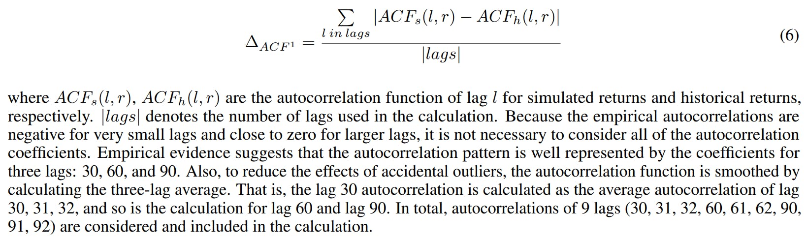
The third part of the stylised facts distance is the difference between simulated and historical autocorrelations of returns. This part in the stylised distance measures the model’s ability to reproduce autocorrelation patterns commonly found in historical returns. It is shown that financial price return time series lack significant autocorrelation, except for short time scales, where significantly negative autocorrelations exist. This phenomenon is backed by our empirical data. For very small lags the autocorrelations are negative, while for larger lags the autocorrelations become insignificant. To measure the distance in autocorrelation patterns between simulated data and historical data, we invoke the autocorrelation function of returns and calculate the average absolute difference between autocorrelations of simulated return time series and historical return time series for various lags:

The last part of the stylised facts distance is the difference between simulated and historical autocorrelations of squared returns. The replication of autocorrelation patterns in squared returns indicates the model’s capability to reproduce the volatility clustering stylised fact. It is shown empirically that large price changes tend to be followed by other large price changes, known as the volatility clustering phenomenon. Consequently, though there are generally no significant patterns in autocorrelations of returns, the autocorrelations of squared returns are significantly positive, especially for small time lags. Also, as time lag increases, the autocorrelation of squared returns displays a slowly decaying pattern, as shown in Figure 2. Similar to the difference between autocorrelations of returns ∆ACF 1 , the difference between autocorrelations of squared returns is calculated as follows:

The above four parts, along with the corresponding weights, constitute the stylised facts distance in Equation (3). The next question is how to determine the associated weight for each part of the stylised facts distance. The basic guiding idea is that the higher the sampling variability of a given part in historical data, the larger the difference between simulated value and historical value that can still be deemed insignificant. A natural candidate for each weight is the inverse of the sampling variance for the corresponding part in the stylised facts distance:

Note that the stylised facts distance is a function of model parameters. In other words, given a set of model parameters, there is a unique stylised facts distance calculated from the simulated time series, which corresponds to that particular set of model parameters. Let θ denote the vector of model parameters to be estimated, Equation (3) can be rewritten as:

[7] Evening trading sessions are excluded. That is, the data span from 8:00 in the morning to 5:00 in the afternoon for each day.