I use Excel’s TAKE and DROP to make top-10 lists that update themselves

Creating top-10 lists in Excel can be tedious if you make them the way I used to. I’d sort the data manually, copy the highest values, and paste them into a separate section. It worked fine, but every time the underlying data changed, I’d have to repeat the entire process. If I missed an update, my report would show outdated information, which isn’t professional when presenting to stakeholders.

That’s where Excel’s TAKE and DROP functions help stop wasting time in Excel. These functions automatically pull the top or bottom items from any dataset and update themselves when the source data changes. So, there’s no more manual copying involved or refreshing reports. While the concept isn’t dramatic, it does eliminate the hassle of manually updating lists.

First, let’s understand dynamic arrays

Before dynamic arrays, a formula’s result was confined to a single cell. To populate a column, you had to drag the fill handle down. Dynamic arrays are different—a single formula can now return an entire range of results that automatically fill multiple cells. This automatic process is called “spilling.” When a formula produces multiple results, they spill into the neighboring blank cells. You’ll know it’s a dynamic array because Excel will draw a thin blue border around the entire output range. This visual cue is your sign that the data is live and connected to the source formula.

You only need to manage the formula in the very first cell of that blue-bordered range. If you try to type something into another cell within the spill area, you’ll get a #SPILL! error. The entire array is controlled by that one initial formula, which makes the sheets cleaner and less prone to errors.

It also applies to the TAKE and DROP functions. Because the results adjust automatically when your source data changes, dynamic arrays obliterate the need to resize tables and manually update results.

Here’s how the TAKE function helps you grab the top items

Credit: Yasir Mahmood /

The TAKE function is designed for a simple task—it extracts a specific number of rows from the beginning or end of a dataset. You just tell Excel how many rows you want instead of manually copying and pasting; it grabs them for you. It is efficient for creating summaries or leaderboards from a larger table.

TAKE uses the following syntax:

=TAKE(array, rows, [columns])

Here’s what the parameters mean:

• array: This is the source range or array of data you want to pull from.
• rows: The number of rows you want to extract. A positive number (like 5) takes from the top, while a negative number (like -5) takes from the bottom.
• [columns]: This is an optional argument. You can specify the number of columns to return from the left (positive number) or right (negative number). If you omit it, TAKE returns all columns.

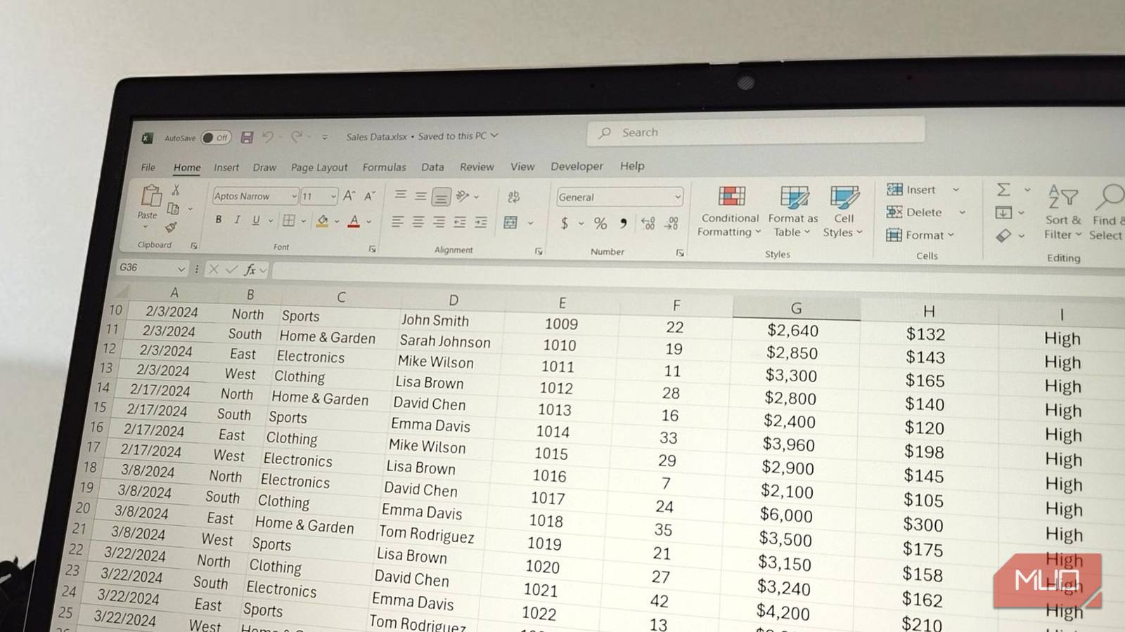
Let’s apply this to a real-world example. Using the sales data, I want to create a dynamic leaderboard showing the top-5 sales amounts.

The key to getting the top performers is first to sort the data from highest to lowest sales. For this, I use the SORT function, which is one of the Excel formulas every office worker should know.

The following formula arranges my entire table based on the seventh column (Sales Amount) in descending order (-1).

=SORT(A2:K33, 7, -1)

Credit: Yasir Mahmood /

With the data sorted, I can now use TAKE to grab only the top five entries. I simply wrap my SORT function inside the TAKE function like this:

=TAKE(SORT(A2:K33, 7, -1), 5)

This single formula first sorts the entire list and then extracts the top 5 rows, creating a self-updating leaderboard. If I change any sales amount in the original table, this list will instantly reflect the new rankings without me having to do anything else.

The DROP function is just as useful for ignoring data you don’t need

Credit: Yasir Mahmood /

The DROP function works as the counterpart to TAKE. Instead of grabbing specific rows, it removes them from your dataset.

It comes in handy when you’re dealing with messy data that includes headers, totals, or irrelevant entries that you need to skip over. Rather than manually selecting around unwanted rows, you tell Excel how many to ignore from the top or bottom.

The syntax mirrors TAKE but with opposite logic:

=DROP(array, rows, [columns])

Here’s what the parameters mean:

• array: The source range or array you want to modify by removing data.
• rows: The number of rows to remove. Positive numbers drop from the top, negative numbers drop from the bottom.
• [columns]: Optional parameter to drop columns from the left (positive) or right (negative). If omitted, all columns remain.

Using the sales data again, let’s say I want to analyze everything except the bottom three performers. Hence, I can use DROP to remove the worst performers.

First, I’ll sort the data to identify the bottom performers:

=SORT(A2:K33, 7, 1)

Credit: Yasir Mahmood /

Notice I’m using (1) instead of (-1) to sort from lowest to highest sales amounts. Now I’ll drop the bottom three rows:

=DROP(SORT(A2:K33, 7, 1), -3)

The negative number tells Excel to remove three rows from the end of the sorted list.

This formula gives me a clean dataset that focuses on everyone except the lowest performers, which is useful for analyzing your core sales team without the outliers skewing your analysis.

I combine them to create more advanced reports

By nesting TAKE and DROP together, you can isolate a specific slice of data from the middle of your ranked list. This is handy for creating tiered reports, like identifying mid-level performers or products that are neither top-sellers nor bottom-dwellers.

Let’s use the same sales data again. We’ve already found the top five and the rest of the list. But what if we only want to see the employees who ranked from 6th to 10th? To achieve this, we use a formula that executes in a specific order from the inside out:

=TAKE(DROP(SORT(A2:K33, 7, -1), 5), 5)

Here’s how Excel processes that request. First, the SORT function arranges the entire table by sales amount in descending order. Then, the DROP function takes that sorted list and removes the top five rows. Afterward, the TAKE function grabs the first five rows from the remaining data, which gives us exactly the 6th-to-10th-place performers.

You can also use this to find underperforming sales without including the absolute worst result. For example, to see the second-to-fifth-worst performers, you can drop the single worst performer from the bottom (-1) and then take the next four from that remaining list. The formula is just a slight variation:

=DROP(TAKE(SORT(A2:K33, 7, 1), 5), 1)

Here, the data is sorted in ascending order (1), the first five rows are taken (5), and then the top-most row is dropped (1).

For a more advanced report, I combine these functions with FILTER to create a leaderboard for a specific region. To find the top three performers in the North region, I first filter the data, then sort it, and then take the top three.

=TAKE(SORT(FILTER(A2:K33, B2:B33="North"), 7, -1), 3)

This formula creates a completely dynamic, region-specific leaderboard. If the sales data changes or if a salesperson moves to a different region, the list will update itself.

I’ll never go back to the old methods

There are plenty of ways to rank data in Excel, but most are either designed for heavy analysis or involve manual steps that just feel clunky. If all I need is a clean, self-updating leaderboard, I don’t have to deal with pivot tables or hard-to-read legacy formulas. The combination of TAKE and DROP provides a much more direct path to the result.

This method is a no-fuss solution that works without needing to be refreshed and uses formulas that are easy for anyone to understand. They’re quick and simple for creating ranked reports that stay current with my data.