I use these 6 Excel array formulas to crush complex calculations

Excel’s basic formulas work fine for simple calculations, but they quickly become cumbersome when you’re dealing with complex data analysis. You end up with nested functions that are hard to read, multiple helper columns cluttering your spreadsheet, and formulas that can break when your data changes. That’s where I use Excel array formulas.

Array formulas let you perform calculations across entire ranges of data in a single formula. Hence, you can handle lightning-fast lookups, filtering, and sorting with just one powerful expression, instead of writing separate formulas for each row or column. They’re not new to Excel, but some people stick with the old ways of doing things when these functions could make their work much simpler and more efficient.

5

XLOOKUP

It beats VLOOKUP every time

XLOOKUP is the lookup function that should have existed from the beginning. Unlike VLOOKUP, which forces you to count columns and only searches to the right, XLOOKUP works in any direction and uses actual column references. It has the following syntax:

=XLOOKUP(lookup_value, lookup_array, return_array, [if_not_found], [match_mode], [search_mode])

Here’s what each parameter means:

• lookup_value: The specific value you’re searching for. This could be a part number, product code, or any identifier in your dataset.
• lookup_array: The range where Excel searches for your lookup_value. It’s typically a single column or row containing your search criteria.
• return_array: The range containing the values you want to retrieve. It can be a single column, multiple columns, or even an entire table section.
• if_not_found (optional): Custom text or value to display when no match exists. It eliminates those annoying #N/A errors and lets you display “Not Found” or “Check Part Number” instead.
• match_mode (optional): Controls the type of match. Use 0 for exact match (default), -1 for exact match or next smallest, 1 for exact match or next largest, and 2 for wildcard matching.
• search_mode (optional): Determines search direction. I use 1 to search first to last (default), -1 searches last to first, and 2 performs binary search on sorted data.

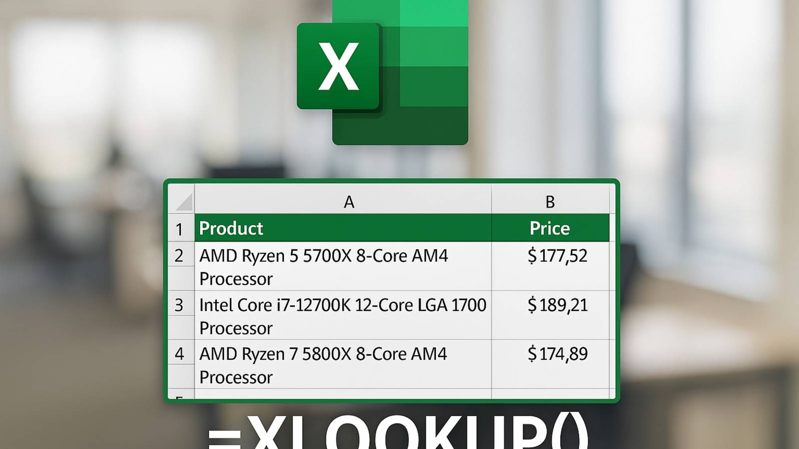
Let’s take an example of a mechanical inventory spreadsheet. The following formula searches for the part number “BRG-002” within the Part IDs range and returns the corresponding data. If the part doesn’t exist, it displays “Part not found” instead of an error.

=XLOOKUP("BRG-002", A:A, A:H, "Part not found")

Yasir Mahmood /

XLOOKUP allows you to pull data from different columns without the column-counting headaches of VLOOKUP, which makes it one of the most important Excel functions for quickly finding data.

4

SUMPRODUCT

The conditional calculation powerhouse

Yasir Mahmood /

SUMPRODUCT doesn’t just add numbers, but it multiplies arrays and then sums the results. This makes it handy for complex conditional calculations that would otherwise require multiple helper columns.

It has the following syntax:

=SUMPRODUCT(array1, [array2], [array3], ...)

Here, array1 is the first range of values to multiply—typically your primary data column, like quantities or costs. And, array2 is an optional second range for multiplication, which often contains criteria or conditional logic using comparison operators.

It becomes even more useful when we use logical operators within the arrays. For example, when we write conditions like (Supplier=”Siemens”), Excel converts the TRUE/FALSE results to 1/0, allowing mathematical operations to proceed.

As an example, the following formula calculates the total inventory value for parts supplied by Siemens only. The formula multiplies quantities by unit costs, but only for rows where the supplier matches the criteria.

=SUMPRODUCT(D2:D100*H2:H100*(G2:G100="Siemens"))

Similarly, the following formula finds the total cost of bearing inventory that’s well-stocked:

=SUMPRODUCT((C2:C100="Bearings")*(D2:D100>=15)*H2:H100)

It applies two conditions simultaneously—category must be “Bearings” and stock levels must be 15 units or higher, helping us identify which bearing categories have adequate inventory coverage.

Yasir Mahmood /

Unlike traditional SUM functions with multiple criteria, SUMPRODUCT doesn’t require complex nested structures because it processes multiple conditions in a single, readable formula. SUM functions in Excel, like SUMIF and SUMIFS, work well for basic conditional sums, but SUMPRODUCT excels when you need to multiply values before summing or handle more complex logical operations.

3

FILTER

Yasir Mahmood /

FILTER extracts rows from your dataset based on conditions you specify. Unlike manual filtering, this function creates dynamic results that automatically update when your source data changes. FILTER has the following syntax:

=FILTER(array, include, [if_empty])

Here’s what each parameter controls:

• array: The entire range of data you want to filter. It includes all columns you want in your results, not just the criteria column.
• include: The logical condition that determines which rows to return—uses comparison operators to create TRUE/FALSE arrays for each row.
• if_empty (optional): To display a custom message when no rows meet your criteria. It prevents #CALC! errors and displays meaningful text like “No matches found.”

It works by evaluating your condition against every row in the array. When the condition returns TRUE, that entire row appears in the filtered results. The following is an example from the mechanical inventory spreadsheet:

=FILTER(A2:H101, (C2:C101="Bearings")*(G2:G101="Timken"))

This formula extracts all rows where the supplier is “Timken” and the category is “Bearings”. The asterisk (*) creates an AND condition by multiplying the logical arrays together.

When you add new data to your source range, using Excel’s FILTER function makes more sense than manual sorting and temporary tables because the filtered results update automatically. This makes it handy for creating live dashboards and reports.

2

UNIQUE

Yasir Mahmood /

UNIQUE pulls distinct values from your data range and automatically avoids duplicates. This function is important if you want to create dropdown lists, analyze data categories, and build summary reports. The syntax is:

=UNIQUE(array, [by_col], [exactly_once])

Here’s how each parameter works:

• array: The range containing the data you want to deduplicate—can be a single column, multiple columns, or an entire table section.
• by_col (optional): FALSE compares rows for uniqueness (default), whereas TRUE compares columns. However, most scenarios use the default row comparison.
• exactly_once (optional): FALSE returns all unique values, including those that appear multiple times (default), and TRUE returns only values that appear exactly once in the dataset.

UNIQUE function evaluates each row or value in your array and returns only the first occurrence of each distinct item. The order matches your original data sequence. Following is an example:

=UNIQUE(G2:G22)

This formula extracts all unique supplier names from the supplier column G and creates a clean list without repetition. I use it to build supplier dropdown menus or summary reports.

You can also use it across the entire table, as shown below:

=UNIQUE(A2:F100)

It returns unique combinations across all columns (A through F), showing distinct inventory records. If two parts have identical values in every column, only one appears in the results.

When working with large datasets, UNIQUE eliminates the tedious process of manual duplicate removal. The dynamic results update when new data arrives, and since UNIQUE creates spill arrays, this approach ends the pain of resizing tables by automatically expanding to accommodate all unique values. I use it to maintain clean reference lists and build reliable data validation ranges.

1

SORT and SORTBY

Arrange your data without touching the original

Yasir Mahmood /

SORT and SORTBY functions organize the data dynamically while keeping the source intact. SORT handles basic sorting by column position, while SORTBY sorts based on values in different columns—giving you more flexibility for complex arrangements.

SORT uses this syntax:

=SORT(array, [sort_index], [sort_order], [by_col])

Here’s what each parameter controls:

• array: The data range you want to sort—includes all columns that should appear in the sorted results.
• sort_index (optional): Column number within the array to sort by. Use 1 for the first column, 2 for the second column, etc. (defaults to 1).
• sort_order (optional): Use 1 for ascending order (default), and -1 for descending order.
• by_col (optional): FALSE sorts by rows (default), TRUE sorts by columns—most scenarios use row sorting.

SORTBY has the following syntax:

=SORTBY(array, by_array1, [sort_order1], [by_array2], [sort_order2], ...)

Its parameters include:

• array: The data range to sort—same as SORT, contains all the columns you want in the results.
• by_array1: The range containing values that determine sort order—can be any column, even outside your main array.
• sort_order1 (optional): 1 for ascending (default), -1 for descending.
• by_array2, sort_order2 (optional): Additional sort criteria for multi-level sorting.

Considering an example from the mechanical inventory spreadsheet, these functions handle real sorting scenarios:

=SORT(A2:H22, 4, -1)

This sorts the entire inventory by stock levels in descending order, showing the highest stock items first. The formula sorts by column 4 (stock levels) while maintaining all row relationships.

I use the SORTBY function instead of SORT for better control over sort criteria and multiple sort levels. As an example, the following formula sorts first by category alphabetically, then by stock levels from highest to lowest within each category.

=SORTBY(A2:H22, C2:C22, 1, D2:D22, -1)

Yasir Mahmood /

Clean Spreadsheets, Smarter Results

Array formulas eliminate the clutter of helper columns and nested functions that make spreadsheets hard to maintain. You get single formulas that handle multiple operations, make the workbooks cleaner, and give a more professional look.

A notable advantage is dynamic functionality, as the results update automatically when source data changes. So, no more manual refreshes or broken formula chains, and your spreadsheets become more reliable for ongoing analysis.

Excel’s array function library keeps expanding beyond these core tools. When I need to consolidate data from multiple sources, I use the VSTACK and HSTACK functions to merge ranges. These functions work together to create powerful data processing workflows that would be impossible with traditional formulas.