When you’re working with data in Excel, certain tasks can feel unnecessarily tedious. Maybe you need to split a column of full names into separate first and last name columns, or combine text from multiple cells with specific separators. These aren’t complex analytical challenges—they’re basic data manipulation tasks that come up regularly.
The good news is that Excel has built-in functions that are designed specifically for these situations. But they often get overlooked because they’re not part of the standard Excel toolkit most people learn, including myself. The functions I’ll cover here aren’t about advanced calculations, but if you find yourself doing repetitive data work, these might just save you some time.
5
TEXTSPLIT
Breaks apart text that’s stuck together
If you’ve ever received a spreadsheet where someone crammed first names, last names, and maybe even middle initials into a single cell, you know the pain of trying to separate that data. TEXTSPLIT handles this exact problem—it takes text from one cell and splits it across multiple columns based on a delimiter you specify.
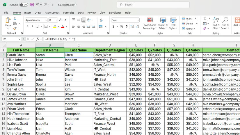
Let’s work with the sample sales data spreadsheet. You’ll see salesperson names listed as “Sarah Chen,” “Mike Johnson,” and “Lisa Park” all in one column. Instead of manually retyping each name into separate columns, TEXTSPLIT can do the work automatically.
It has the following syntax:
=TEXTSPLIT(text, col_delimiter, [row_delimiter], [ignore_empty], [match_mode], [pad_with])
Here’s what each parameter does:
- text: The cell containing the text you want to split.
- col_delimiter: The character that separates your data (like a space, comma, or semicolon).
- row_delimiter (Optional): Used when splitting into both rows and columns.
- ignore_empty (Optional): TRUE ignores empty values, FALSE keeps them (default is FALSE).
- match_mode (Optional): Controls case sensitivity (0 for case-sensitive, 1 for case-insensitive).
- pad_with (Optional): What to fill empty cells with when results have uneven lengths.
For the salesperson names, for example, I would use the following formula to split names into separate columns:
=TEXTSPLIT(A2, " ")
The function automatically creates as many columns as needed based on your data. While this basic approach works for most situations, there are additional parameters that give you precise control over the TEXTSPLIT function in Excel.
4
TEXTJOIN
Combines multiple cells into one
TEXTJOIN does the opposite of TEXTSPLIT. It takes text from multiple cells and combines them into a single cell with whatever separator you choose. This comes in handy when you need to create concatenated values like complete addresses, product descriptions, or email lists.
The syntax looks like this:
=TEXTJOIN(delimiter, ignore_empty, text1, [text2], ...)
Here’s what each parameter controls:
- delimiter: The character or text that separates your joined values (comma, space, hyphen, etc.).
- ignore_empty: TRUE skips blank cells, FALSE includes them in the result.
- text1, text2, etc.: The cells or ranges you want to combine (you can reference individual cells or entire ranges).
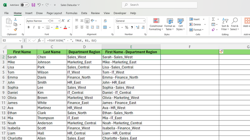
Looking at the sales data spreadsheet, if I have separate columns for first name and department region, but I need them in a single column that combines both, I’ll use TEXTJOIN. Setting ignore_empty to TRUE means any empty cells get skipped automatically.
=TEXTJOIN(" - ", TRUE, B2, D2)
When deciding between different text combination methods, understanding the differences between the CONCAT and TEXTJOIN functions can help you pick the right tool for your specific data joining needs.
3
CHOOSECOLS
Selects specific columns from your data
CHOOSECOLS lets you extract specific columns from a range without copying and pasting or creating references. If you have a large dataset but only need columns two, five, and eight for your analysis, this function grabs what you want and ignores the rest.
From the sales data, I might want to pull just the salesperson names and sales while skipping the order dates, product categories, and other details. Instead of manually selecting and copying columns, CHOOSECOLS creates a dynamic reference that updates automatically when the source data changes.
It has the following syntax:
=CHOOSECOLS(array, col_num1, [col_num2], ...)
Here’s how each parameter works:
- array: The range or table containing your source data (can be a cell range like A1:F100 or a table reference).
- col_num1: The first column number you want to extract (1 for the first column, 2 for the second, etc.).
- col_num2, etc.: Additional column numbers you wish to include (optional—you can specify as many as needed).
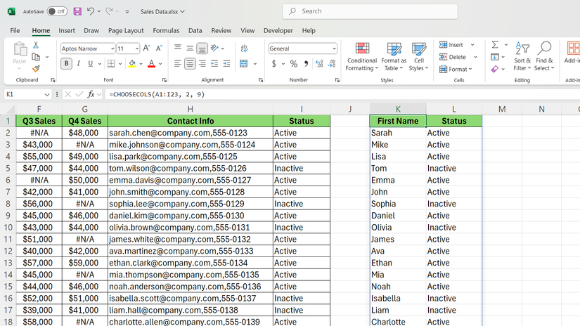
As an example, if I wanted to extract salesperson names from column two and their status from column nine, I would use:
=CHOOSECOLS(A1:I23, 2, 9)
The function returns both columns as a spill array, automatically sizing to fit the data. This is why CHOOSECOLS is one of the Excel functions that can save significant time. It eliminates the need for multiple VLOOKUP formulas or manual column copying when you’re working with large datasets.
Excel also has a CHOOSEROWS function, which works identically but selects specific rows instead of columns, using the same syntax structure with row numbers.
2
TAKE and DROP
TAKE and DROP work as a pair to grab specific portions of your data range. TAKE extracts a certain number of rows or columns from the beginning or end of your dataset, while DROP removes rows or columns from the beginning or end, leaving you with what remains.
These functions work as precision tools for data sampling. If you need just the first ten rows of data for a quick analysis, or want to remove header rows that are cluttering your calculations, these functions handle the job cleanly.
TAKE uses this syntax:
=TAKE(array, rows, [columns])
DROP follows a similar pattern:
=DROP(array, rows, [columns])
Here’s how the parameters work for both functions:
- array: The source data range you want to extract from or modify.
- rows: Number of rows to take/drop (positive numbers work from the top, negative from the bottom).
- columns (Optional): Number of columns to take/drop (positive from left, negative from right).
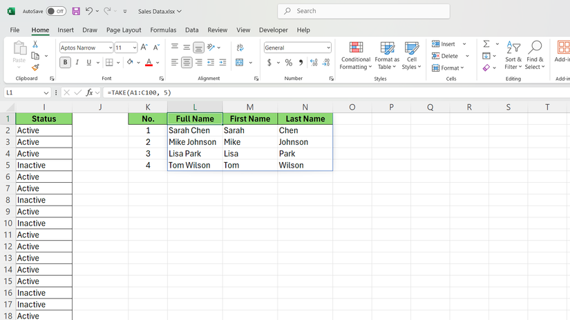
To get the first five rows from the sales data, use the following formula:
=TAKE(A1:C100, 5)
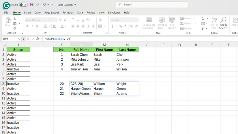
To remove the top twenty rows and work with clean data, try:
=DROP(A1:C23, 20)
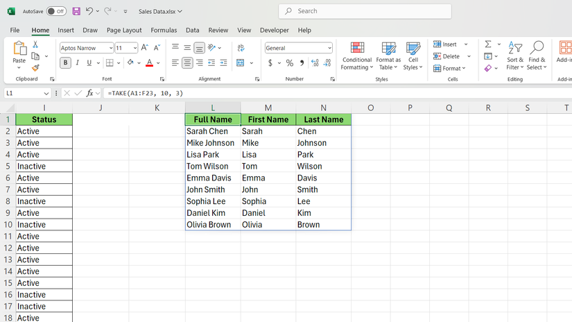
You can combine both row and column operations. For instance, the following formula gives you the first ten rows and first three columns:
=TAKE(A1:F23, 10, 3)
These functions come in handy, especially when you need dynamic data subsets that adjust automatically. Learning how to use the TAKE and DROP functions in Excel opens up possibilities for creating flexible reports that adapt to changing dataset sizes.
1
AGGREGATE
Powerful calculations that handle messy data
AGGREGATE combines the functionality of 19 different statistical functions into one flexible formula. What makes it special is its ability to ignore errors, hidden rows, or filtered data—something standard functions like SUM or AVERAGE can’t do reliably.
If your data contains some #N/A error, or if you’ve filtered to show only specific regions, AGGREGATE can calculate totals, averages, or other statistics without those issues throwing off your results. I find it useful when working with dynamic datasets where visibility and data quality change frequently.
The syntax includes several components:
=AGGREGATE(function_num, options, array, [k])
Each parameter controls different aspects of the calculation:
- function_num: A number from 1-19 that specifies which function to use (1=AVERAGE, 4=MAX, 9=SUM, 12=MEDIAN, etc.).
- options: Controls what to ignore during calculation (0=nothing, 1=hidden rows, 2=error values, 3=hidden rows and errors, 5=error values only, 6=hidden rows and error values).
- array: The range of cells to perform the calculation on.
- k (Optional): Used only with certain functions like LARGE, SMALL, or PERCENTILE.
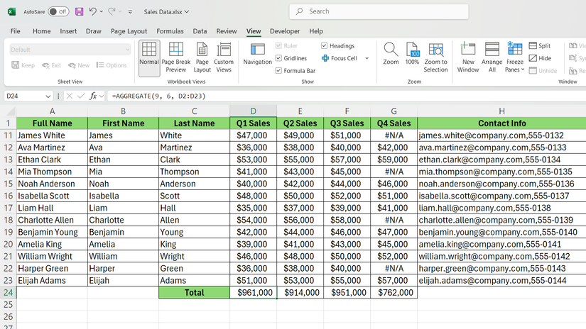
To sum visible sales amounts while ignoring any errors, I would use:
=AGGREGATE(9, 6, D2:D23)
The number 9 specifies SUM, and 6 tells it to ignore both hidden rows and error values.
This kind of robust calculation capability is exactly why AGGREGATE belongs among the Excel formulas every office worker should know—it handles real-world data messiness that simpler functions can’t manage effectively.
Built-in tools worth using
Excel’s most valuable functions often aren’t the ones people learn first. Yet they handle the exact problems that come up in real spreadsheet work, including messy text data, extracting specific portions of large datasets, and performing calculations on imperfect data. None of the functions we discussed require advanced Excel skills. However, TEXTSPLIT, CHOOSECOLS, TAKE, and DROP are only available in Microsoft 365 and Excel for the web.
The next time you find yourself doing repetitive data cleanup or manually copying columns, remember these functions exist. They’re already built into Excel to handle the boring stuff, so you can focus on what the data actually tells you.

