Researchers Use Diffusion Models To Simulate DOOM Gameplay In Real Time

Table of Links

ABSTRACT

1 INTRODUCTION

2 INTERACTIVE WORLD SIMULATION

3 GAMENGEN

3.1 DATA COLLECTION VIA AGENT PLAY

3.2 TRAINING THE GENERATIVE DIFFUSION MODEL

4 EXPERIMENTAL SETUP

4.1 AGENT TRAINING

4.2 GENERATIVE MODEL TRAINING

5 RESULTS

5.1 SIMULATION QUALITY

5.2 ABLATIONS

6 RELATED WORK

7 DISCUSSION, ACKNOWLEDGEMENTS AND REFERENCES

2 INTERACTIVE WORLD SIMULATION

An Interactive Environment E consists of a space of latent states S, a space of partial projections of the latent space O, a partial projection function V : S → O, a set of actions A, and a transition probability function p(s|a, s′ ) such that s, s′ ∈ S, a ∈ A. For example, in the case of the game DOOM, S is the program’s dynamic memory contents, O is the rendered screen pixels, V is the game’s rendering logic, A is the set of key presses and mouse movements, and p is the program’s logic given the player’s input (including any potential non-determinism). Given an input interactive environment E, and an initial state s0 ∈ S, an Interactive World Simulation is a simulation distribution function q(on|o ment and the simulation when enacting the agent’s policy π. Importantly, the conditioning actions for these samples are always obtained by the agent interacting with the environment E, while the conditioning observations can either be obtained from E (the teacher forcing objective) or from the simulation (the auto-regressive objective). We always train our generative model with the teacher forcing objective. Given a simulation distribution function q, the environment E can be simulated by auto-regressively sampling observations.

3 GAMENGEN

GameNGen (pronounced “game engine”) is a generative diffusion model that learns to simulate the game under the settings of Section 2. In order to collect training data for this model, with the teacher forcing objective, we first train a separate model to interact with the environment. The two models (agent and generative) are trained in sequence. The entirety of the agent’s actions and observations corpus Tagent during training is maintained and becomes the training dataset for the generative model in a second stage. See Figure

3. 3.1 DATA COLLECTION VIA AGENT PLAY

Our end goal is to have human players interact with our simulation. To that end, the policy π as in Section 2 is that of human gameplay. Since we cannot sample from that directly at scale, we start by approximating it via teaching an automatic agent to play. Unlike a typical RL setup which attempts to maximize game score, our goal is to generate training data which resembles human play, or at least contains enough diverse examples, in a variety of scenarios, to maximize training data efficiency. To that end, we design a simple reward function, which is the only part of our method that is environment-specific (see Appendix A.3). We record the agent’s training trajectories throughout the entire training process, which includes different skill levels of play. This set of recorded trajectories is our Tagent dataset, used for training the generative model (see Section 3.2).

3.2 TRAINING THE GENERATIVE DIFFUSION MODEL

We now train a generative diffusion model conditioned on the agent’s trajectories Tagent (actions and observations) collected during the previous stage. We re-purpose a pre-trained text-to-image diffusion model, Stable Diffusion v1.4 (Rombach et al., 2022). We condition the model fθ on trajectories T ∼ Tagent, i.e. on a sequence of previous actions a<n and remove all text conditioning. Specifically, to condition on actions, we simply learn an embedding Aemb from each action (e.g. a specific key press) into a single token and replace the cross attention from the text into this encoded actions sequence. In

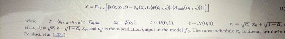
Figure 4:Auto-regressive drift. Top: we present every 10th frame of a simple trajectory with 50 frames in which the player is not moving. Quality degrades fast after 20-30 steps. Bottom: the same trajectory with noise augmentation does not suffer from quality degradation.

order to condition on observations (i.e. previous frames) we encode them into latent space using the auto-encoder ϕ and concatenate them in the latent channels dimension to the noised latents (see Figure 3). We also experimented conditioning on these past observations via cross-attention but observed no meaningful improvements. We train the model to minimize the diffusion loss with velocity parameterization (Salimans & Ho, 2022b):

3.2.1 MITIGATING AUTO-REGRESSIVE DRIFT USING NOISE AUGMENTATION

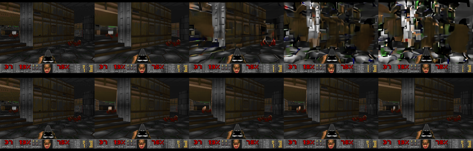
The domain shift between training with teacher-forcing and auto-regressive sampling leads to error accumulation and fast degradation in sample quality, as demonstrated in Figure 4. To avoid this divergence due to auto-regressive application of the model, we corrupt context frames by adding a varying amount of Gaussian noise to encoded frames in training time, while providing the noise level as input to the model, following Ho et al. (2021). To that effect, we sample a noise level α uniformly up to a maximal value, discretize it and learn an embedding for each bucket (see Figure 3). This allows the network to correct information sampled in previous frames, and is critical for preserving frame quality over time. During inference, the added noise level can be controlled to maximize quality, although we find that even with no added noise the results are significantly improved. We ablate the impact of this method in section 5.2.2.

3.2.2 LATENT DECODER FINE-TUNING

The pre-trained auto-encoder of Stable Diffusion v1.4, which compresses 8×8 pixel patches into 4 latent channels, results in meaningful artifacts when predicting game frames, which affect small details and particularly the bottom bar HUD (“heads up display”). To leverage the pre-trained knowledge while improving image quality, we train just the decoder of the latent auto-encoder using an MSE loss computed against the target frame pixels. It might be possible to improve quality even further using a perceptual loss such as LPIPS (Zhang et al. (2018)), which we leave to future work. Importantly, note that this fine tuning process happens completely separately from the U-Net finetuning, and that notably the auto-regressive generation isn’t affected by it (we only condition autoregressively on the latents, not the pixels). Appendix A.2 shows examples of generations with and without fine-tuning the auto-encoder.

3.3 INFERENCE 3.3.1 SETUP

We use DDIM sampling (Song et al., 2022). We employ Classifier-Free Guidance (Ho & Salimans, 2022) only for the past observations condition o<n. We didn’t find guidance for the past actions condition a<n to improve quality. The weight we use is relatively small (1.5) as larger weights create artifacts which increase due to our auto-regressive sampling.

We also experimented with generating 4 samples in parallel and combining the results, with the hope of preventing rare extreme predictions from being accepted and to reduce error accumulation. We experimented both with averaging the samples and with choosing the sample closest to the median. Averaging performed slightly worse than single frame, and choosing the closest to the median performed only negligibly better. Since both increase the hardware requirements to 4 TPUs, we opt to not use them, but note that this might be an interesting area for future work.

3.3.2 DENOISER SAMPLING STEPS

During inference, we need to run both the U-Net denoiser (for a number of steps) and the autoencoder. On our hardware configuration (a TPU-v5), a single denoiser step and an evaluation of the auto-encoder both takes 10ms. If we ran our model with a single denoiser step, the minimum total latency possible in our setup would be 20ms per frame, or 50 frames per second. Usually, generative diffusion models, such as Stable Diffusion, don’t produce high quality results with a single denoising step, and instead require dozens of sampling steps to generate a high quality image. Surprisingly, we found that we can robustly simulate DOOM, with only 4 DDIM sampling steps (Song et al., 2020). In fact, we observe no degradation in simulation quality when using 4 sampling steps vs 20 steps or more (see Appendix A.4). Using just 4 denoising steps leads to a total U-Net cost of 40ms (and total inference cost of 50ms, including the auto encoder) or 20 frames per second. We hypothesize that the negligible impact to quality with few steps in our case stems from a combination of: (1) a constrained images space, and (2) strong conditioning by the previous frames.

Since we do observe degradation when using just a single sampling step, we also experimented with model distillation similarly to (Yin et al., 2024; Wang et al., 2023) in the single-step setting. Distillation does help substantially there (allowing us to reach 50 FPS as above), but still comes at a some cost to simulation quality, so we opt to use the 4-step version without distillation for our method (see Appendix A.4). This is an interesting area for further research. We note that it is trivial to further increase the image generation rate substantially by parallelizing the generation of several frames on additional hardware, similarly to NVidia’s classic SLI Alternate Frame Rendering (AFR) technique. Similarly to AFR, the actual simulation rate would not increase and input lag would not reduce.

:::info
Authors: